Find Common Items Across Multiple Columns in Google Sheets

This tutorial explains how to find common items across multiple columns in Google Sheets. It’s one of those super useful techniques you should master.

Wondering why? Let’s first see where it comes into play in real life. Once you understand the use cases, you’ll be excited to learn this trick without any further ado!

What Do “Common Items” Mean?

Imagine you have five lists across columns A, B, C, D, and E.

If an item appears in all these columns, that’s considered a common item.

Our goal is to create a formula that can search across multiple columns and extract all the common items — in one go.

Real-Life Use Cases

Here are a few practical situations where finding common items across columns becomes handy:

1. Student Enrollment Across Courses

You have lists of students enrolled in different classes (e.g., Column A = Math, Column B = Science, Column C = History).

You want to find students enrolled in all courses.

2. Product Listings on Multiple Platforms

Your business sells products on Amazon, Shopify, and Etsy.

You want to find products listed on all platforms.

3. Event Registrations

You organized multiple workshops (e.g., Column A = Workshop 1 attendees, Column B = Workshop 2 attendees).

You want to find participants who signed up for multiple workshops.

4. Consolidating Survey Responses

Different teams collected survey responses separately.

You want to find people who responded to more than one survey.

Formula to Find Common Items Across Multiple Columns in Google Sheets

To find common items across multiple columns in Google Sheets, you can use the following formula:

=LET(
   rlist, FILTER(range, BYCOL(range, LAMBDA(dVal, COUNTA(dVal)))), 
   list, TOCOL(BYCOL(rlist, LAMBDA(col, UNIQUE(col))), 3), 
   rc, ARRAYFORMULA(COUNTIFS(list, list, SEQUENCE(ROWS(list)), "<="&SEQUENCE(ROWS(list)))), 
   SORT(FILTER(list, rc=COLUMNS(rlist)))
)

Important:

Replace range with your actual range reference.

Let’s see how to apply this formula step-by-step with a sample dataset.

Features of This Formula

It’s an array formula, meaning it returns all results in one go.
It automatically ignores empty columns, which is super useful when your data has blank separators between lists.
(Without this feature, a blank column would cause an error!)
You can even use the extracted list to highlight common items across columns in Google Sheets.

Example: Finding Common Students Enrolled in Multiple Courses

1. Set Up the Data

Let’s say you manage enrollments for different classes. Here’s your data across columns A, B, and C:

Math	Science	History
Janie	Lewis	Janie
Lewis	Charlie	Latasha
Charlie	Janie	Lewis
David	Latasha	Frank
Latasha	David	Charlie
Stephen		Wesley
		Lance

You want to find students enrolled in all three courses.

2. Applying the Formula

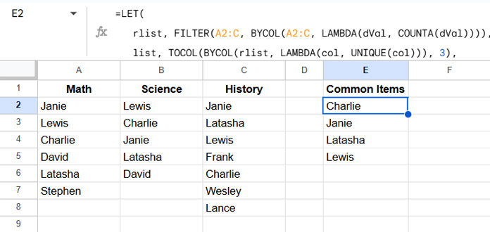
Enter the following formula to find the common names:

=LET(
   rlist, FILTER(A2:C, BYCOL(A2:C, LAMBDA(dVal, COUNTA(dVal)))), 
   list, TOCOL(BYCOL(rlist, LAMBDA(col, UNIQUE(col))), 3), 
   rc, ARRAYFORMULA(COUNTIFS(list, list, SEQUENCE(ROWS(list)), "<="&SEQUENCE(ROWS(list)))), 
   SORT(FILTER(list, rc=COLUMNS(rlist)))
)

It will return the students who are enrolled in all three classes.

Example of finding common items across multiple columns in Google Sheets

Formula Logic and Explanation

Here’s how the formula works behind the scenes:

rlist:
=FILTER(A2:C, BYCOL(A2:C, LAMBDA(dVal, COUNTA(dVal))))
Filters out any completely empty columns.
list:
=TOCOL(BYCOL(rlist, LAMBDA(col, UNIQUE(col))), 3)
Uniques each column, then arranges them into a single column.
rc:
=ARRAYFORMULA(COUNTIFS(list, list, SEQUENCE(ROWS(list)), "<="&SEQUENCE(ROWS(list))))
Counts how often each item appears as we go down the list.
SORT(FILTER(list, rc = COLUMNS(rlist))):
Filters the items that appear as many times as there are non-empty columns, meaning they are common to all.

Highlighting Common Items Across Multiple Columns

Once you’ve found the items that appear in all columns, highlighting them is a piece of cake!

Suppose your common items list is in E1:E.

Here’s how to highlight the matching values across A1:C:

Select the range A1:C.
Go to Format > Conditional formatting.
Under Format Rules, choose Custom formula is.
Enter the following formula:
=XMATCH(A1, $E$1:$E)
Choose your formatting style and click Done.

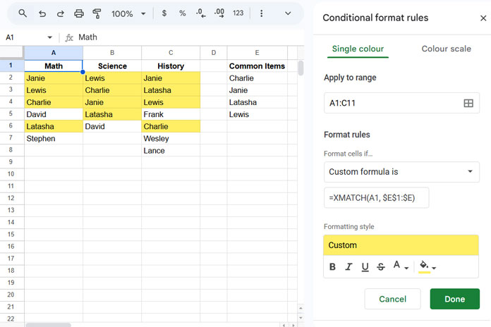
Highlighting items that appear in all columns in the range

Now, all the common items across your columns will be highlighted.

The items that are not highlighted are those that do not appear in all columns.