


")


")

")
")
 in Excel & Google Sheets")


This tutorial explains how to filter the bottom 10 items in a Pivot Table in Google Sheets. Mastering this technique can be valuable in various real-world scenarios. For example, you can use it to identify the 10 lowest-selling products, helping businesses focus on improving sales strategies. It can also be useful for tracking the 10 least-used vehicles in a fleet, allowing for better resource allocation. Additionally, this method can highlight the 10 least-visited tourist destinations, offering insights for marketing or infrastructure improvements.
Why Use a Custom Formula?
Google Sheets does not provide a built-in option to filter the bottom 10 items in a Pivot Table. To achieve this, you need to use a custom formula. The formula will vary depending on whether you are grouping by a single column or multiple columns.
Before we begin, it’s essential to understand tie-breaking modes, which determine how to handle cases where multiple items share the same value at the cutoff.
Tie-Breaking in Bottom 10 Filtering in a Pivot Table
| Tie-Breaking Mode | Description |
| 0 | Strictly Bottom N |
| 1 | Bottom N + duplicates of the Nth occurrence (if any) |
| 2 | Unique Bottom N |
| 3 | Bottom N + all duplicates |
In the formula, you can select your preferred tie-breaking mode by adjusting the mode number. Let’s look at an example to clarify how each mode works.
Example: Understanding Tie-Breaking Modes
Here’s a sample vehicle log, where we identify the three least-used vehicles:
| Vehicle ID | Distance Traveled (km) | Mode 0 (Strict Bottom 3) | Mode 1 (Bottom 3 + Duplicates) | Mode 2 (Unique Bottom 3) | Mode 3 (Bottom 3 + All Duplicates) |
| V001 | 100 | ✅ | ✅ | ✅ | ✅ |
| V002 | 100 | ✅ | ✅ | ✅ | |
| V003 | 300 | ✅ | ✅ | ✅ | ✅ |
| V004 | 300 | ✅ | ✅ | ||
| V005 | 800 | ✅ | ✅ | ||
| V006 | 800 | ✅ | |||
| V007 | 1200 |
Example 1: Filter the Bottom 10 Items in a Pivot Table (Single Column Grouping)
Use this sample sheet to explore both single-column and multi-column bottom 10 filtering in a Pivot Table.
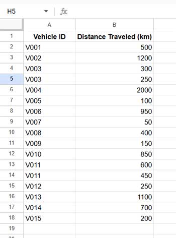
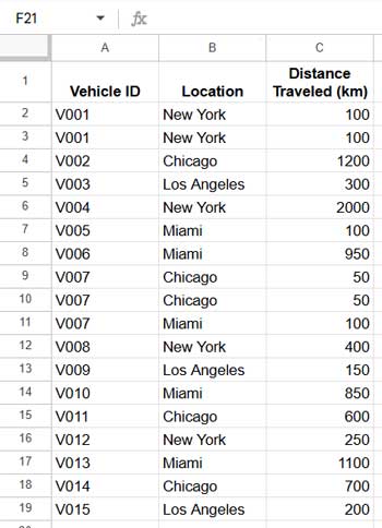
Sample Data (Sheet1)
Creating the Pivot Table
Follow these steps to create a Pivot Table:
- Select A1:B
- Go to Insert > Pivot Table
- In the popup window, click Create to place the Pivot Table in a new sheet
- Drag Vehicle ID under Rows
- Drag Distance Traveled (km) under Values and set it to SUM
- In the Vehicle ID field, sort by SUM of Distance Traveled (km) in Ascending order
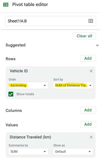
This will group the data by vehicle and sort it with least-used vehicles at the top.
Formula to Filter the Bottom 10 Items in a Pivot Table
=XMATCH('Vehicle ID', CHOOSECOLS(SORTN(QUERY(QUERY(Sheet1!A1:B, "select Col1, sum(Col2) where Col1 is not null group by Col1 order by sum(Col2)"), "offset 1", 0), 10, 0, 2, TRUE), 1))Modifications You Need to Make:
- Replace Vehicle ID with your actual field label
- Replace Sheet1!A1:B with the source data range
- Change 0 (the first zero from right to left) to your preferred tie-breaking mode (0-3)
Applying the Formula in the Pivot Table
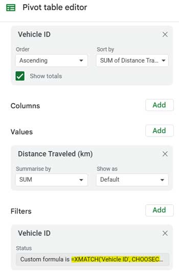
- In the Pivot Table editor, drag Vehicle ID under Filters
- Click on the filter field (currently showing “All items”)
- Select Filter by Condition > Custom formula is
- Copy and paste the modified formula
- Click OK
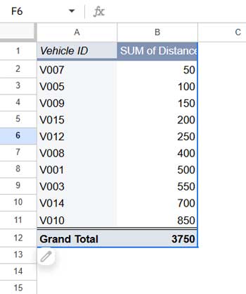
This will filter the Pivot Table to display only the 10 least-used vehicles.
Example 2: Filter the Bottom 10 Items in a Pivot Table (Multi-Column Grouping)
Sample Data (Sheet2)
Creating the Pivot Table with Two-Column Grouping
To create a Pivot Table for filtering the bottom 10 items when grouping by Vehicle ID and Location, follow these steps:
- Select the data range
A1:Cin Sheet2. - Go to Insert > Pivot Table and click Create to insert it into a new sheet.
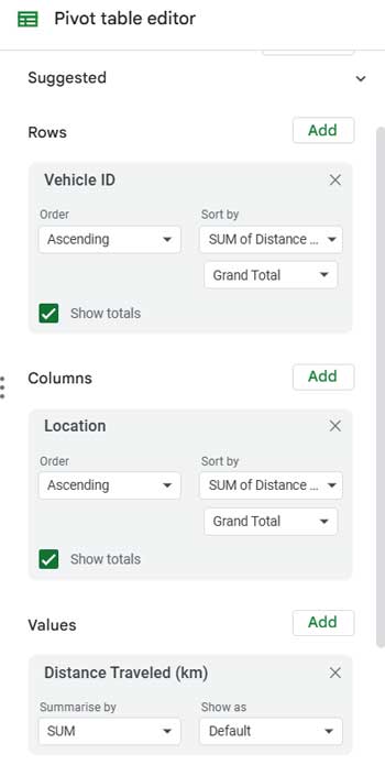
- In the Pivot Table editor:
- Drag Vehicle ID under Rows.
- Drag Location under Columns.
- Drag Distance Traveled (km) under Values and set it to SUM.
- In both Rows and Columns, select Sort by > SUM of Distance Traveled (km) and choose Ascending order.
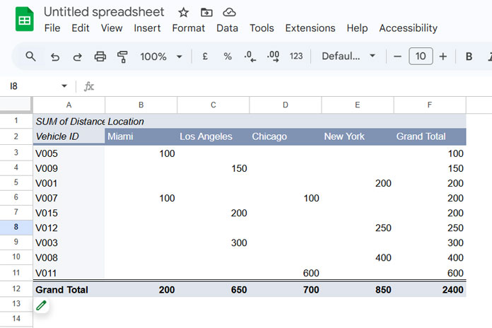
This will generate a Pivot Table grouped by both Vehicle ID and Location, sorting vehicles based on their total traveled distance.
Now, we can apply the formula to filter the bottom 10 items from this Pivot Table.
Formula to Filter the Bottom 10 Items (Multi-Column Grouping)
=XMATCH('Vehicle ID'&Location, LET(sN, SORTN(QUERY(QUERY(Sheet2!A1:C, "select Col1, Col2, sum(Col3) where Col1 is not null group by Col1, Col2 order by sum(Col3)"), "offset 1", 0), 10, 0, 3, TRUE), ARRAYFORMULA(HSTACK(CHOOSECOLS(sN, 1)&CHOOSECOLS(sN, 2)))))Modifications You Need to Make:
- Replace Vehicle ID & Location with your actual field labels
- Update Sheet2!A1:C with your data range
- Adjust the tie-breaking mode (0-3)
Applying the Formula
- Drag Vehicle ID under Filters in the Pivot Table editor.
- Select Filter by condition > Custom formula is and paste the formula.
- Click OK to apply the filter.
Replacing Bottom 10 with Bottom 3, 5, or N
To filter the bottom 3, bottom 5, or any N items, simply replace 10 in the formula with your desired number. This works for both single-column and multi-column grouping.
Why Use a Pivot Table Instead of QUERY?
While QUERY can return the bottom N items, it lacks:
- Grand Totals, which require additional steps in QUERY.
- Advanced Tie-Breaking, which requires combining SORTN with QUERY for proper handling.
Using a Pivot Table with a custom formula is a better, scalable approach.
Note: The custom formula does use QUERY and SORTN, but it is designed to be easy for users to modify.
Final Thoughts
I hope this tutorial helps you effectively filter the bottom 10 items in a Pivot Table in Google Sheets. If you have questions, feel free to comment below!