If you ask me what is the solution to exclude 0 from MIN function result in Google Sheets, my answer would be either by using a Filter function or a QUERY function together with MIN. The MIN formula alone can’t perform this task.

Here in this quick Google Sheets tips, I’m detailing the above two different methods to return minimum value that without 0 in Google Doc Spreadsheets.

Steps to Exclude 0 From MIN Function Result in Google Sheets

As I told you above, there are two different options. Let’s begin with Filter with MIN.

Filter with MIN to Exclude Zero

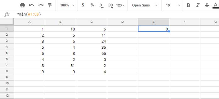
When you have the values to test for MIN excluding zero is properly arranged in Columns, Rows or as a data range, you can use the FILTER function with MIN.

Obviously, the above MIN function is returning 0. So here is the formula using Filter to return MIN value excluding 0.

I’m going to filtered out 0 from each column and then join them vertically, i.e., data of one column under another, and use the MIN function as usual then. See that formula below.

=min({filter(A1:A8,A1:A8<>0);filter(B1:B8,B1:B8<>0);filter(C1:C8,C1:C8<>0)})

If there is only a single column, you can avoid using Curly Braces. One Single Filter formula is enough for them.

Query with MIN to Exclude Zero

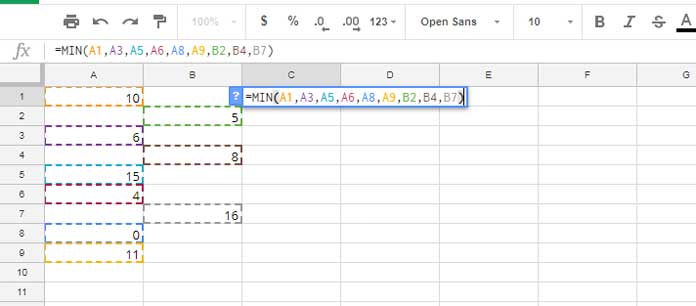
When the values to test for MIN excluding 0 are scattered in different cells and columns, the possibly best option is to use Query with MIN.

The above MIN formula would, of course, return the result 0. Below is the Query alternative to returning minimum value without 0 from the scattered values in Google Sheets.

=min(query({A1;A3;A5;A6;A8;A9;B2;B4;B7},"select * where Col1<>0"))

Formula Explanation:

The curly braces make the scattered values as an array means a single column. As you know, we can use a column in Query function as data to filter. Hope you can read the above formula as it’s a straightforward approach.

This way you can exclude 0 from MIN function result in Google Sheets. If you have any doubt about using the above functions, please do post in comments below. I will find time to answer your questions. That’s all for now.