I have a spreadsheet with content in a foreign language. How can I read it? It’s possible! You can detect and translate content in Google Sheets using its built-in functions.
Open your spreadsheet in Google Sheets and use the functions DETECTLANGUAGE and GOOGLETRANSLATE in combination. These are two individual Google Sheets functions that make it easy to translate content directly within your spreadsheet.
Why Combine These Functions?
Most of the time, it can be challenging to identify the foreign language you want to translate. Even if you manage to figure it out, you’ll need to know the corresponding language code.
The DETECTLANGUAGE function identifies the language code for you, which can then be used within the GOOGLETRANSLATE function. However, this step is optional because GOOGLETRANSLATE has a built-in option to automatically detect the language and translate the content to your specified language.
Let’s dive into how these functions work.
How to Use the DETECTLANGUAGE Function in Google Sheets
Syntax:
DETECTLANGUAGE(text_or_range)- text_or_range: This can be hardcoded text or a reference to a cell containing the text to evaluate. You can also refer to a one-dimensional range, in which case the function will identify the language of the very first cell in that range. Make sure the first cell is not empty.
Example of the DETECTLANGUAGE Function:
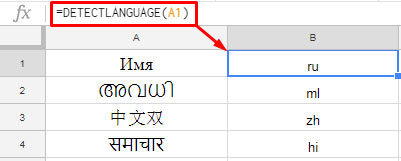
Suppose you have text in column A, starting from cell A1. Use the following formula in cell B1 and drag it down:
=DETECTLANGUAGE(A1)
If you want to detect the language of a range, use this:
=DETECTLANGUAGE(A1:A5)In this case, the formula will detect the language of the text in the first cell of the range (A1).
How to Use the GOOGLETRANSLATE Function in Google Sheets
Since the topic is about how to detect and translate content in Google Sheets, let’s now look at the translation process.
Syntax:
GOOGLETRANSLATE(text, [source_language, target_language])- text: Hardcoded text or a cell reference to the text you want to translate.
- source_language: The language code of the source text. If you don’t know this, you can either use the DETECTLANGUAGE function or set it to
"auto". - target_language: The language code for the desired translation.
You can omit both source_language and target_language to allow the function to detect the source language and translate the text to your spreadsheet’s default language.
Example:
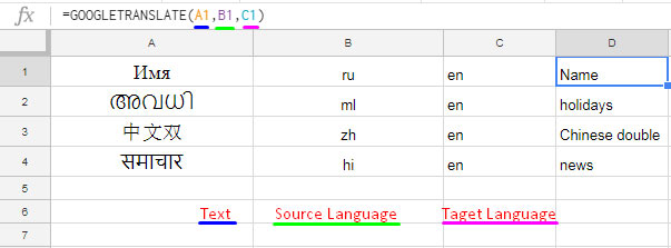
If the texts to translate are in A1:A4, the source language codes are in B1:B4, and the target language codes are in C1:C4, enter the following formula in cell D1 and drag it down to translate all the texts:
=GOOGLETRANSLATE(A1, B1, C1)
Detect and Translate Content in Google Sheets: Combined Formula
Here’s how you can combine the two functions to detect and translate content in Google Sheets:
Formula:
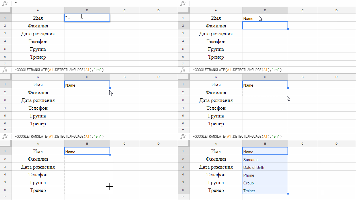
=GOOGLETRANSLATE(A1, DETECTLANGUAGE(A1), "en")
This formula uses the output of the DETECTLANGUAGE function as the source language and translates the text into English ("en").
Alternatively:
You can simplify this by using "auto" to let GOOGLETRANSLATE automatically detect the language:
=GOOGLETRANSLATE(A1, "auto", "en")To translate text into your spreadsheet’s default language, use:
=GOOGLETRANSLATE(A1)Language Codes for the GOOGLETRANSLATE Function
You can find a full list of language codes for use with GOOGLETRANSLATE on the Google Developers Language Codes page. To import them into your sheet, use this IMPORTHTML formula in cell A1 of an empty sheet:
=IMPORTHTML("https://developers.google.com/admin-sdk/directory/v1/languages", "table", 1)Conclusion
By combining DETECTLANGUAGE and GOOGLETRANSLATE, you can efficiently detect and translate content in Google Sheets. Whether you’re working with a single cell or a large dataset, these functions make handling multilingual content seamless.
If you want an array formula, you can use the MAP lambda helper function. The generic formula is:
=MAP(range, LAMBDA(text, GOOGLETRANSLATE(text, "auto", "en")))Replace range with the range containing the text you want to translate.
Follow the tips above to streamline your workflow and simplify translation tasks!


