


")


")

")
")
 in Excel & Google Sheets")


How to Calculate the Number of Interest Payments (Coupons) Between the Settlement and Maturity Dates of an Investment, Such as a Bond
To calculate the number of interest payments, also known as coupons, between the settlement date and maturity date of an investment (like a bond), we can use the COUPNUM function in Google Sheets.
Required Parameters for the COUPNUM Function
In addition to the settlement and maturity dates, you need to know the frequency of the coupon payments. There are three possible frequencies:
- Annual (1)
- Semiannual (2)
- Quarterly (4)
Another factor that will affect the calculation is the day count basis to follow.
COUPNUM Function – Syntax and Arguments
Syntax:
COUPNUM(settlement, maturity, frequency, [day_count_convention])Arguments:
- settlement: The settlement date of the security, which refers to the date after issuance when the security is traded to the buyer.
- maturity: The maturity or expiration date of the security.
- frequency: The number of coupon payments per year (refer to table #1 below).
- day_count_convention: An optional argument that indicates the day count basis to follow (refer to table #2 below)
Table #1 – Frequency
| Frequency Indicator | Coupon (COUPNUM) Basis |
| 1 | Annual |
| 2 | Semiannual |
| 4 | Quarterly |
Table #2 – Day Count Basis
| Day Count Indicator | Day Count Basis |
| 0 or omitted | US 30/360 (as per NASD standards) |
| 1 | Actual/Actual |
| 2 | Actual/360 |
| 3 | Actual/365 |
| 4 | European 30/360 (according to European conventions) |
COUPNUM Function Example in Google Sheets
Here is an example of how to use the COUPNUM function in Google Sheets.
In the following example, cells B2, B3, B4, and B5 contain the settlement date, maturity date, frequency, and day count convention, respectively.
=COUPNUM(B2, B3, B4, B5)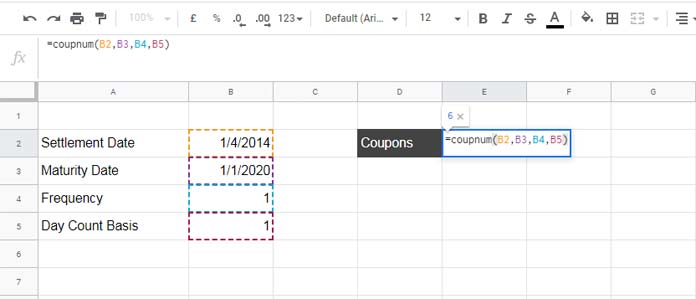
Based on the above settlement date, maturity date, and day count basis, the semiannual coupon numbers (COUPNUM) will be 12, while the quarterly coupon numbers will be 23. You can verify this by changing the frequency in cell B4 to 2 (for semiannual) or 4 (for quarterly).
Important Points to Note
How to Properly Input the Settlement and Maturity Dates
To quickly calculate the number of coupons, you may use the COUPNUM function as follows:
=COUPNUM("2014-4-1", "2020-1-1", 4, 1)While this method allows you to avoid cell references for the arguments, it is not recommended. Instead, in all functions, particularly those in the financial category, it’s best to use the DATE function for date inputs.
When you are not using cell references in the COUPNUM formula, you should write it as follows:
=COUPNUM(DATE(2014, 4, 1), DATE(2020, 1, 1), 4, 1)Here, the DATE function follows this syntax: =DATE(year, month, day).
Error Values in the COUPNUM Function in Google Sheets
The COUPNUM function may return the #VALUE! error in the following scenarios:
- Invalid settlement date
- Invalid maturity date
For example, if the default date format in your sheet is dd/mm/yyyy, but you accidentally enter the settlement or maturity date in mm/dd/yyyy format, you may see the #VALUE! error or incorrect coupon numbers.
The COUPNUM function may return the #NUM! error in the following cases:
- If the frequency is any number other than 1, 2, or 4 (out of range)
- If the day count basis is less than 0 or greater than 4 (out of range)
- If the settlement date is greater than or equal to the maturity date
That’s all about using the COUPNUM function in Google Sheets. Enjoy!