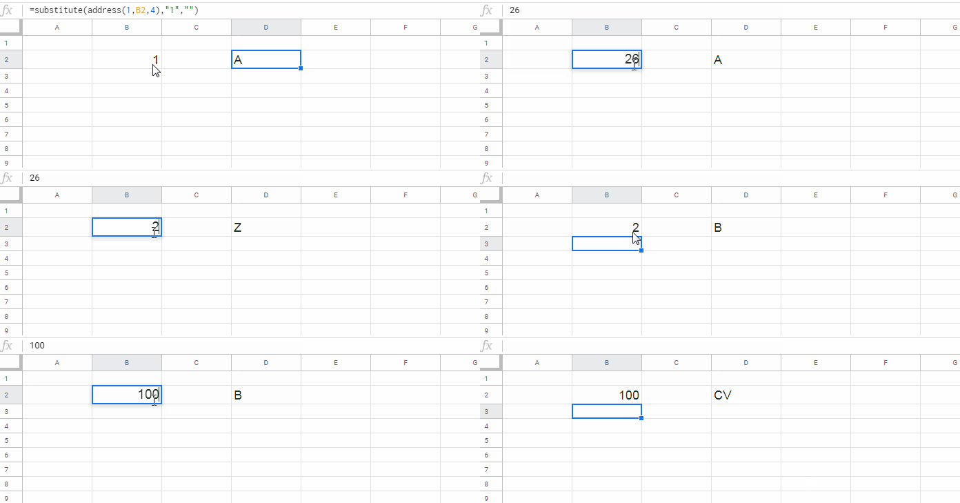
Using the ADDRESS and REGEXEXTRACT functions, you can get a column letter from a given column number in Google Sheets. However, this isn’t the only way to do it.
Another effective method involves using the ADDRESS function along with SUBSTITUTE instead of REGEXEXTRACT. Not only do these methods differ, but their underlying logic also varies.
Furthermore, I’ve included instructions on how to convert a column letter to a column number, essentially the reverse process, in Google Sheets.
Formula to Convert a Given Column Number to its Corresponding Column Letter
I have mentioned two combinations, right? Here they are:
Generic Formula 1:
=REGEXEXTRACT(ADDRESS(1, column_number_to_convert), "[A-Z]+")Feed the column_number_to_convert with the required column number. For example, if you input 26, the formula will return the column letter “Z”.
Example:
=REGEXEXTRACT(ADDRESS(1, 26), "[A-Z]+")
Explanation:
The ADDRESS formula returns the cell reference “$Z$1” using the input values, which are row number (1) and column number (26).
Syntax of the ADDRESS Function: ADDRESS(row, column, [absolute_relative_mode], [use_a1_notation], [sheet])
If we can remove the characters “$” and “1” from the output, we have achieved our goal! I mean, we have converted column number 26 to the corresponding column letter “Z”.
Instead of removing the unwanted characters from the ADDRESS formula output, I have used REGEXEXTRACT to extract the required letter “Z”.
The regular expression "[A-Z]+" will discard any characters other than the letters A-Z from the output.
Syntax of the REGEXEXTRACT Function: REGEXEXTRACT(text, regular_expression)
We can also use SUBSTITUTE with ADDRESS to convert a provided column number to the corresponding column letter in Google Sheets. This is a different approach and a favorite of Excel users.
Generic Formula 2:
=SUBSTITUTE(ADDRESS(1, column_number_to_convert, 4), "1", "")Example:
=SUBSTITUTE(ADDRESS(1, 26, 4), "1", "")Explanation:
This is a quite different approach. Here the ADDRESS formula returns “Z1” instead of “$Z$1” because I have used the optional argument, absolute_relative_mode, #4 in the formula.
As a result of this, other than the column letter (column identifier), the only character left with the output is the row number “1”.
We can substitute the row number “1” with “” to get the column letter from the column number.
Syntax of the SUBSTITUTE Function: SUBSTITUTE(text_to_search, search_for, replace_with, [occurrence_number])
Formula to Convert a Given Column Letter to its Corresponding Column Number
Before learning how to get a column number from a column letter, let me explain why this formula will be very helpful in Google Sheets.
If you use the QUERY function, you may know that it accepts both column letters and column numbers as identifiers.
For example:
=QUERY(A1:G, "Select F")
=QUERY({A1:G}, "Select Col6")
The above two formulas perform the same task, which is selecting only column F (the 6th column) from columns A to G.
However, you can’t use the column letter ‘BY’ in QUERY because it’s a reserved word. For instance, the formula below won’t work:
=QUERY(A1:BY, "Select BY")The solution is to use the column number instead of the column letter in the formula.
Let’s see how to convert a column letter like ‘BY’ or any other column letter to a column number in Google Sheets.
Generic Formula:
=COLUMN(INDIRECT("column_letter_to_convert"&1))Example:
=COLUMN(INDIRECT("BY"&1))Explanation:
The COLUMN function returns the column number of a cell reference. If you specify =COLUMN(BY1) or =COLUMN(INDIRECT("BY1")), it will return the column number 77.


