How about changing the tick box/checkbox color while toggling in Google Sheets? I want the color of the tick box to turn red when the status is checked. How can I do that?

If this is your question, just read on. Here, you can learn how to change the tick box color while toggling in Google Sheets.

The tick box is one of the relatively recent additions to Google Sheets, available in the Insert menu as well as in the Data menu under Data validation.

To change the tick box color, you can rely on the conditional formatting feature in Google Sheets. No coding knowledge is required!

With conditional formatting, you can change the tick box color in Google Sheets.

In this tutorial, I am sharing two different options: one formula and one preset rule for formatting the tick box.

1. The highlighting rule to change the tick box color while toggling in Google Sheets.
2. Conditional formatting formula to change the row color when the tick box is checked.

How to Change the Tick Box Color While Toggling in Google Sheets?

Here are the two examples.

Example 1: The Highlighting Rule to Change the Tick Box Color While Toggling in Google Sheets

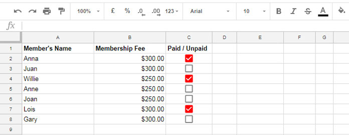
In this example, you can observe that the color of the ticked tick boxes is red.

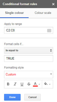
To achieve this, follow the conditional formatting settings outlined below:

1. Navigate to the very first cell in the range containing the tick box (e.g., C2).
2. Access the conditional formatting menu: Format > Conditional formatting.
3. Configure the custom formatting based on the provided screenshot.

In short:

• In the Conditional Format Rules panel, “Apply to range” is the range where you want to apply the highlighting. It’s the range C2:C8 in my example.
• Select “Is equal to” under “Format cells if…” and enter the Boolean value TRUE in the field below that.
• Choose Text color under the formatting style. My preferred color formatting is red for Text color and white for Fill color.

Example 2: Conditional Formatting Formula to Change the Row Color When the Tick Box is Ticked

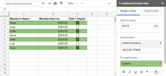
When you want to highlight the row when the tick box is toggled (ticked), you must use a custom formula in Google Sheets.

In the above example, the “Apply to range” is C2:C8. Please check the screenshot above. Here we will select A2:C8 since we want the highlighting to change the row color.

Formula:

=$C2=TRUE

or

=$C2:$C=TRUE

Within the Conditional Format Rules panel, under “Format cells if…”, select “Custom formula is” and enter either of the above formulas.

Select your preferred Text and Fill colors.

The Logic Behind the Tick Box Color Changes

The logic behind the above two types of conditional formatting is simple.

By default, the value of the cell containing the tick box is the Boolean FALSE. When ticked, it changes to TRUE. This change in value can be utilized to format the cells or rows containing the tick box or the tick box itself.

Sometimes, the value of the tick box is not necessarily the Boolean TRUE or FALSE because Google Sheets permits changing the default tick box value. You can check whether the value of the tick box is TRUE or FALSE in the following way.

Suppose your cell C2 has one tick box. In another blank cell, apply the below formula.

=C2

This will return the value of the tick box.

If you want to learn more about how to insert the tick box in Google Sheets and change the default Boolean TRUE or FALSE value, you can follow my tutorial below.

Must Read: Insert CheckBox, Tick Mark in Google Sheets

I hope you now understand how to change the tick box color while toggling in Google Sheets. Make your Sheet stunning. Enjoy!