How to Calculate Digital Root in Google Sheets

The digital root is the single-digit value you get by repeatedly summing the digits of a number until only one digit remains. For instance, the digital root of 942 is:

9 + 4 + 2 = 15 → 1 + 5 = 6

In this tutorial, you’ll learn how to calculate the digital root in Google Sheets using simple formulas—no script or add-on needed.

What’s the Point of Digital Roots?

You might think digital roots are just a cool math trick—but they’re actually used in more places than you’d expect:

Quick Math Checks: Ever heard of “casting out nines”? It’s a shortcut to check if long calculations are likely correct.
Numerology & Life Path Numbers: Big in numerology—people use it to analyze names and birthdates.
Modulo 9 Shortcut: The digital root is basically MOD(n, 9), with a small tweak to turn 0 into 9.
Teaching Tool: Great for explaining number patterns, divisibility rules, and mental math in a fun way.
Games & Puzzles: Some number-based puzzles and games use digital roots in their logic or scoring systems.

Calculate the Digital Root of a Single Number

If your number is in cell A1, use the following formula to calculate its digital root:

=MOD(A1 - 1, 9) + 1

How This Formula Works:

A1 - 1: Handles numbers like 9, 18, 27 (multiples of 9) that would otherwise result in 0.
MOD(..., 9): Finds the remainder after dividing by 9.
+ 1: Corrects 0 to 9, giving you a result from 1 to 9.

Example – Digital Root of 3636

If A1 = 3636, the calculation is:

3 + 6 + 3 + 6 = 18 → 1 + 8 = 9
The formula gives the same result: MOD(3635, 9) + 1 = 8 + 1 = 9

You get the digital root in a single step!

Note: To find the digital root of a date (for example, in cell A1), use this formula:

=MOD(TEXT(A1, "DDMMYYYY") - 1, 9) + 1

This converts the date to a continuous number string (day, month, year) and calculates its digital root.

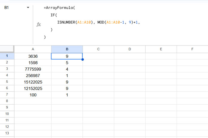
Calculate Digital Roots for a Range

To find the digital roots of multiple numbers in a column (e.g., A1:A10), use:

=ArrayFormula(
   IF(
      ISNUMBER(A1:A10), MOD(A1:A10 - 1, 9) + 1,
   )
)

This will return the digital roots for each cell in the range automatically.

Example of calculating digital root in Google Sheets

Show Both Stages of the Digital Root

If you’d like to display both the first-stage digit sum and the final digital root, you can use:

=LET(
  digits, SPLIT(REGEXREPLACE(A1 & "", "(\d)", "$1,"), ","),
  stage1, SUM(digits),
  stage2, MOD(stage1 - 1, 9) + 1,
  HSTACK(stage1, stage2)
)

What This Formula Does:

stage1: Sums all digits (e.g., 3 + 6 + 3 + 6 = 18)
stage2: Final digital root (e.g., 1 + 8 = 9)
HSTACK: Displays the two results side-by-side

You can replace HSTACK with VSTACK if you prefer the results in a vertical layout.

This method is useful when you’re analyzing number breakdowns for checksum validation, numerology, or educational purposes.

Frequently Asked Questions (FAQ)

Q1: What is a digital root?
A digital root is the single-digit number obtained by repeatedly summing the digits of any number until only one digit remains. For example, the digital root of 942 is 6 because 9 + 4 + 2 = 15, and 1 + 5 = 6.

Q2: How do I calculate the digital root in Google Sheets?
You can calculate the digital root in Google Sheets using the formula =MOD(A1-1, 9)+1 where A1 is the cell with your number. This formula returns the single-digit digital root efficiently without using scripts.

Q3: Can I calculate the digital root of a date in Google Sheets?
Yes! Convert the date to a continuous number string with TEXT(A1, "DDMMYYYY") and then use the formula =MOD(TEXT(A1, "DDMMYYYY") - 1, 9) + 1 to get its digital root.

Q4: Why is the digital root useful?
Digital roots help in error checking calculations (like casting out nines), numerology, teaching number patterns, and even some puzzle and game logic.

Q5: Can I calculate digital roots for multiple numbers at once in Google Sheets?
Absolutely! Use an ArrayFormula like this:
=ArrayFormula(IF(ISNUMBER(A1:A10), MOD(A1:A10 - 1, 9) + 1,))
This calculates digital roots for all numbers in the range A1:A10.