XLOOKUP is a modern lookup function in Excel, and when combined with HYPERLINK, it can serve two useful purposes:

• Jump to a cell where the XLOOKUP result is located.
• Return a clickable hyperlink that directs to an external website or file.

In this tutorial, you’ll learn how to use XLOOKUP with HYPERLINK in both scenarios with easy-to-follow examples.

Jump to a Cell Using XLOOKUP and HYPERLINK in Excel

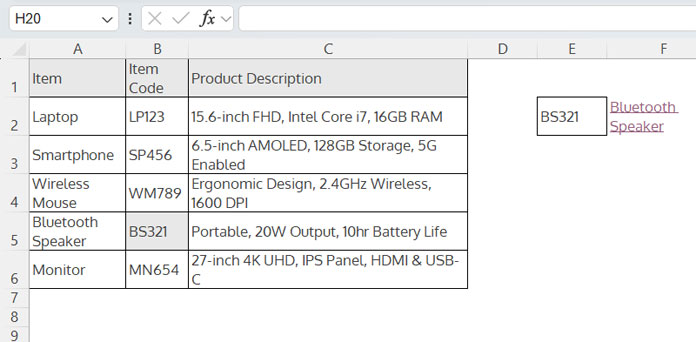
In the following example, we have columns for Item, Item Code, and Product Description. Our goal is to look up an item code, return the corresponding item, and jump to the cell containing that item. This allows for quick verification and modification of the product description if needed.

Steps to Use XLOOKUP with HYPERLINK to Jump to the Result Cell

1. Enter the lookup value in any cell, for example, BS321 in E2.
2. Use the following formula in F2 to return the corresponding item name:
   =XLOOKUP(E2, B2:B6, A2:A6)
   This formula searches for E2 in B2:B6 and returns the corresponding product from A2:A6.
3. Wrap it with the CELL function to get the cell address:
   =CELL("address", XLOOKUP(E2, B2:B6, A2:A6))
4. Add the “#” sign to create an internal link:
   ="#" & CELL("address", XLOOKUP(E2, B2:B6, A2:A6))
5. Wrap it with HYPERLINK to generate a clickable link:
   =HYPERLINK("#" & CELL("address", XLOOKUP(E2, B2:B6, A2:A6)))
6. Optionally, replace the cell address with the product name as the link text:
   =HYPERLINK("#" & CELL("address", XLOOKUP(E2, B2:B6, A2:A6)), XLOOKUP(E2, B2:B6, A2:A6))

This method allows you to jump to the XLOOKUP result cell using HYPERLINK in Excel.

Optimized Formula Using LET

To avoid repeating the XLOOKUP calculation, use the LET function:

=LET(xl, XLOOKUP(E2, B2:B6, A2:A6), HYPERLINK("#"&CELL("address", xl), xl))

When using this formula:

• Replace E2 with the search key.
• Replace B2:B6 with your lookup range.
• Replace A2:A6 with your result range.

Return a Clickable Link to a Website or External File Using XLOOKUP

If the XLOOKUP result range contains a hyperlink, XLOOKUP loses the link and returns plain text. (As a side note, this is not the case with XLOOKUP in Google Sheets.)

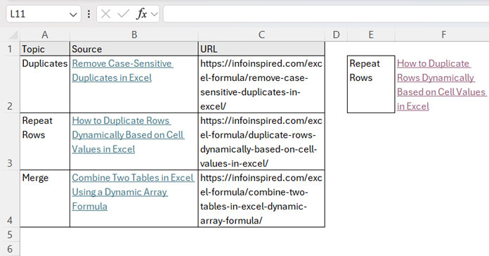
To retain the link, the best approach is to maintain a separate column with the URLs of the external sources.

Sample Table:

Steps to Create a Clickable Link Using XLOOKUP

1. Use the following formula to look up the topic and return the text (without a hyperlink):
   =XLOOKUP(E2, A2:A4, B2:B4)
2. Instead of the result text, return the URL from the third column:
   =XLOOKUP(E2, A2:A4, C2:C4)
3. Wrap it with HYPERLINK to create a clickable link:=HYPERLINK(XLOOKUP(E2, A2:A4, C2:C4))

When you click this link, it will open the corresponding webpage in your browser.

Looking Up and Opening Files Stored on Your Computer

If you want to link to a file stored on your computer, specify the file path in the result range instead of a URL. For example:

C:\Users\HP\OneDrive\Pictures\Screenshots\Screenshot 2024-11-24 114433.png

The formula remains the same:

=HYPERLINK(XLOOKUP(E2, A2:A4, C2:C4))

Clicking the link will open the specified file.

Resources

• How to Jump to the Current Date Cell in Excel
• Excel: Jump to the VLOOKUP Result Cell