


")


")

")
")
 in Excel & Google Sheets")


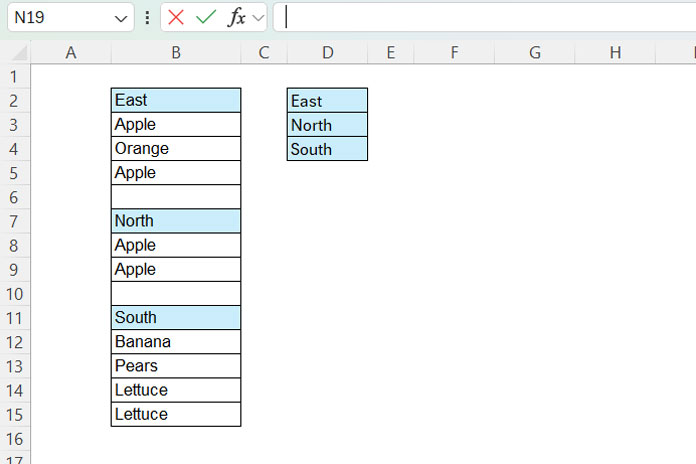
If you have a list in a column separated by categories, you might want to extract unique items by section (category) in Excel. This can be done using a dynamic array formula.
The category labels define each section. In the following list, the sections are separated by regions: East and North.
East
Apple
Orange
Apple
North
Apple
Apple
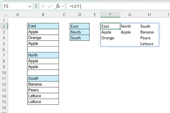
We would expect the section-wise unique values to appear as follows:
East
Apple
Orange
North
Apple
While this task involves LAMBDA functions, don’t let that deter you from using the formula. You specify the range and category, and the formula handles the rest. You can also choose to omit the detailed formula explanation at the end of the tutorial.
Note: You can achieve a similar result as shown below, where unique items are retained, and duplicates are removed in a column next to the source data. I’ll include this in a separate section titled “Additional Tips” at the end.
| East | East |
| Apple | Apple |
| Orange | Orange |
| Apple | – |
| – | – |
| North | North |
| Apple | Apple |
| Apple | – |
Here’s how to create a unique list within sections of a column in Excel.
Step 1: Creating a Category List
Assume the data is in column B, range B2:B15.
From that list, you should extract the categories and enter them in column D. For example, if the categories that determine the sections are East, North, and South, enter them in D2:D4.
You don’t need to enter all the categories. Only enter the categories for which you want to extract the section-wise unique values.
Step 2: Applying the Formula to Create a Unique List by Section
Enter the following formula in cell F2:
=LET(
   category, D2:D4,
   range, TOCOL(B2:B15, 1),
   group,
      SCAN(0, IFNA(XMATCH(range, category), ""),
         LAMBDA(a, v, IF(v="", a, v))
      ),
   DROP(IFNA(
      REDUCE("", UNIQUE(group),
         LAMBDA(aA, vV, HSTACK(aA, UNIQUE(FILTER(range, group=vV))))
      ), ""), 0, 1
   )
)
When you use this formula to create a unique list by section breaks in a column, make the following changes:
- Replace
D2:D4with your category range. - Replace
B2:B15with your source data range.
Step 3: Removing the Helper Column
You can remove the helper column (D2:D4) by specifying the categories as a constant array using the VSTACK function, as follows:
You can replace D2:D4 with VSTACK("East", "North", "South").
How Does the Formula Generate a Unique List by Section in Excel?
Feel free to skip this formula explanation if you're new to Excel's LAMBDA functions and dynamic arrays.
The key functions in this Excel formula are SCAN and REDUCE, which work together to extract unique lists by section from data in a column.
SCAN Part (Named as ‘group’ using the LET function):
SCAN(0, IFNA(XMATCH(range, category), ""), LAMBDA(a, v, IF(v="", a, v)))Where:
rangeisTOCOL(B2:B15, 1)(which removes empty cells) andcategoryisD2:D4
(Both names, i.e., “range” and “category,” are defined using the LET function)
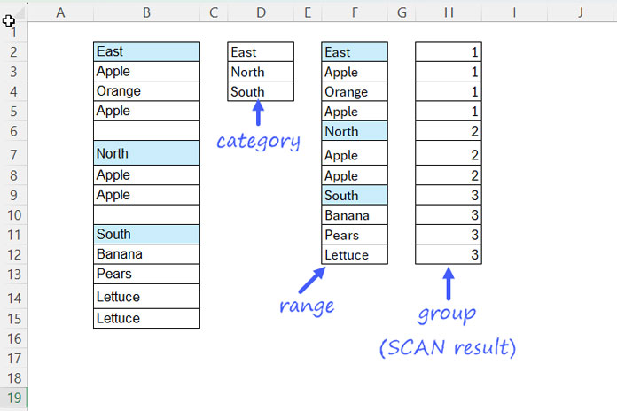
In this part, XMATCH matches the range against the category and assigns positions to the categories. The section breaks will get the sequence numbers 1, 2, and 3, while the values under the categories will return #N/A. IFNA removes these #N/A errors.
The purpose of SCAN is to fill the blank cells in the output by carrying forward the last non-blank value from above. This assigns a section number to each value.
REDUCE Part:
REDUCE("", UNIQUE(group), LAMBDA(aA, vV, HSTACK(aA, UNIQUE(FILTER(range, group=vV)))))Here, FILTER(range, group=vV) filters the range where group matches each element in the array UNIQUE(group). The REDUCE function iterates through each element (vV) in the array.
The intermediate results are horizontally stacked using the HSTACK function to combine the unique lists by section.
IFNA removes #N/A errors, and DROP removes the empty column that results from using an empty string (initial value in the accumulator, i.e., aA) in the REDUCE function and stacking the results using the HSTACK function.
The final result is a unique list for each section.
Additional Tip: Displaying Unique Lists by Section Side by Side in Excel
You can follow this approach if you don’t want to move the unique lists to separate category columns.
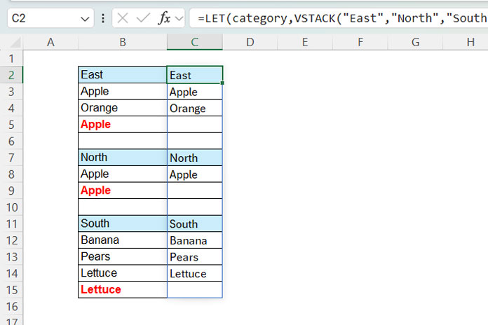
In this method, the formula scans the lists in column B and returns the output in column C, removing duplicates by section.
This is another way to create a unique list within sections of a column in Excel.
Formula:
=LET(
   category, VSTACK("East", "North", "South"),
   range, B2:B15,
   group,
      SCAN(0, IFNA(XMATCH(range, category), ""),
         LAMBDA(a, v, IF(v="", a, v))
   ),
   rc,
      SORTBY(
         SEQUENCE(ROWS(range&group), 1, 2)-MATCH(SORT(range&group),
         SORT(range&group), 0), SORTBY(SEQUENCE(ROWS(range&group), 1, 2
      ), range&group, 1), 1),
   IF(rc=1, IF(range="", "", range), " ")
)
When you use this formula, replace B2:B15 with the source range that contains the list separated by categories in a column. Also, replace "East", "North", and "South" with the categories that define each section.
Formula Explanation:
The first part of the formula, i.e., up to the SCAN part, is taken from our previous formula that creates unique lists by section, placing them in their own columns.
Up to the SCAN function, the formula assigns a sequence to each section — for example, 1 for all values in the first section, 2 for the second section, and so on.
Instead of using REDUCE, here we use a SORTBY formula that returns the running count of range&group, which combines the values in the range B2:B with the SCAN output (group). Here’s that part:
SORTBY(SEQUENCE(ROWS(range&group), 1, 2)-MATCH(SORT(range&group), SORT(range&group), 0), SORTBY(SEQUENCE(ROWS(range&group), 1, 2), range&group, 1), 1)The assigned name is rc, and the second column in the table below reflects the output of rc.
| East | 1 |
| Apple | 1 |
| Orange | 1 |
| Apple | 2 |
| 1 | |
| North | 1 |
| Apple | 1 |
| Apple | 2 |
| 1 | |
| South | 1 |
| Banana | 1 |
| Pears | 1 |
| Lettuce | 1 |
| Lettuce | 2 |
Finally, the IF(rc=1, IF(range="", "", range), " ") part removes duplicates based on sections, producing the output in column C.
If rc=1 and B2:B is not blank, the formula returns the values from B2:B; otherwise, it returns an empty string.