
")
")


")


")

")
")
 in Excel & Google Sheets")


Sorting by last name in Excel is useful in various real-world scenarios, especially when managing lists of names in professional or organizational settings.
For example, if your organization generates email addresses based on last names, sorting by last name ensures consistency. Similarly, in HR databases or event registration lists, sorting by last name makes it easier to find individuals.
In this tutorial, I’ll show you how to sort names by last name in Excel using a formula—without relying on helper columns. We’ll use the SORTBY and REGEXEXTRACT functions. Since these functions are available in Excel 365 and later versions, check for compatibility before using them.
Sample Data
The sample data consists of ten names in B2:B11, though you can use this approach for a larger list.
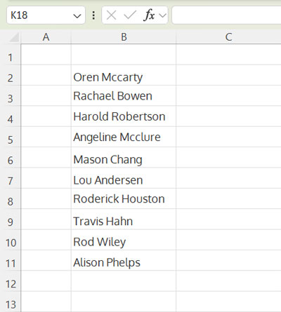
We will apply the formula in C2 to arrange these names by last name in ascending order.
Formula to Sort by Last Name in Excel
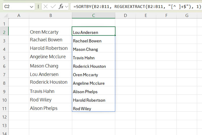
Once your names are listed in B2:B11, use the following formula in C2:
=SORTBY(B2:B11, REGEXEXTRACT(B2:B11, "[^ ]+$"), 1)This formula sorts the names by last name in ascending order.
If you want to sort by last name in descending order, simply replace 1 (the last argument) with -1:
=SORTBY(B2:B11, REGEXEXTRACT(B2:B11, "[^ ]+$"), -1)Formula Explanation
1. Extracting the Last Name Using REGEXEXTRACT
=REGEXEXTRACT(B2:B11, "[^ ]+$")This formula extracts the last name from each full name using a regular expression (REGEX).
Understanding the REGEX pattern
[^ ]: A negated character class that matches any character that is not a space.+: A quantifier that matches one or more occurrences of non-space characters.$: An anchor that matches the end of the string.
In simple terms, this pattern captures the last word (the last name) in each cell.
2. Using SORTBY to Sort the Names by Last Name
The SORTBY function sorts data dynamically based on another range.
Syntax of SORTBY:
=SORTBY(array, by_array1, [sort_order1], [by_array2, sort_order2], …)- array: The list of names to sort (
B2:B11). - by_array1: The extracted last names (
REGEXEXTRACT(B2:B11, "[^ ]+$")). - sort_order1: The sorting order (
1for ascending,-1for descending).
This formula dynamically sorts the full names based on extracted last names.
Handling Trailing Zeros in the Sorted List
If you reference a larger range (e.g., B2:B100) and some rows are empty, the formula might return trailing zeros (0s) in the output.
To remove trailing zeros, use the following LET-based formula:
=LET(
   last_name, REGEXEXTRACT(B2:B100,"[^ ]+$"),
   sorting, SORTBY(B2:B100,last_name,1),
   IF(sorting=0,"",sorting)
)
How this works:
LETassigns the extracted last names to last_name.- The
SORTBYfunction sorts the full names based on last_name. IF(sorted_data=0, "", sorted_data)replaces any trailing zeros with blank cells.
Simply replace B2:B100 with the actual range containing names.
Conclusion
In this tutorial, you learned a formula-based approach to sorting names by last name in Excel—without using helper columns.
Key Benefits of This Method:
- No Helper Columns Needed – Works directly within a single formula.
- Dynamic Sorting – Automatically updates when new names are added.
- More Efficient – Avoids complex helper column workarounds.
If you need a static sorted list, copy the results, right-click > Paste Special > Values to preserve the order.