


")


Want to sort your Excel data by column names instead of column positions? Learn how to dynamically sort by field labels in Excel using the powerful SORT and XMATCH combo in Excel—no more manual lookups or helper columns! This guide walks you through practical examples, from static field label sorting to fully dynamic dropdown-based sorting.
Why Use the SORT and XMATCH Combo in Excel?
This approach is helpful in several scenarios:
- You don’t need to manually determine the column index to sort.
- It sticks to the correct column even if you move it within the table.
- You can dynamically control the sort column(s) using drop-down lists.
Note: The formula works in Excel versions that support the XMATCH and SORT functions, as well as dynamic arrays (Excel 365 and Excel 2021 and later).
Examples: Sort by Field Labels in Excel
The SORT and XMATCH combo in Excel varies slightly depending on whether you want to sort by a single field label or multiple field labels.
Sample Data (A1:C5):
| Name | Department | Sales |
| Samuel | HR | 5000 |
| Julia | Finance | 7000 |
| Prashanth | IT | 6500 |
| Amalia | HR | 4800 |
1. Sort by a Single Field Label
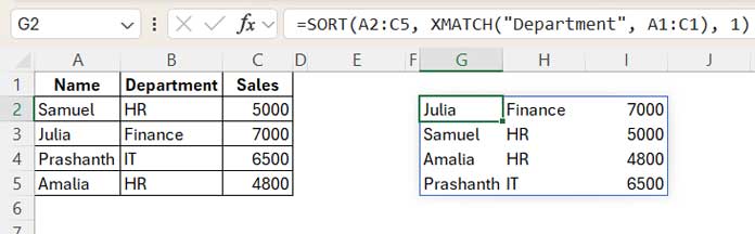
To sort by the field label “Department”, use this formula:
=SORT(A2:C5, XMATCH("Department", A1:C1), 1)A2:C5is the range to sort (array).XMATCH("Department", A1:C1)returns the column index of the field label.1indicates ascending sort order.
This aligns with the syntax:
SORT(array, [sort_index], [sort_order], [by_col])2. Sort by Multiple Field Labels
To sort by both Department and Sales, use:
=SORT(A2:C5, XMATCH({"Department","Sales"}, A1:C1), {1,1})- You pass an array of field labels:
{"Department","Sales"}. - You also pass a corresponding array for sort order:
{1,1}(ascending).
This ensures that sorting happens by Department first, then by Sales.
Sort by Field Label Selected via Drop-down List
To make sorting more interactive, use drop-downs to let users select the sort field(s).
Example: Sort by One Drop-down Selection
- Create a drop-down in cell
E1:- Go to the Data tab → Data Validation.
- Choose List.
- Set the Source to:
=A1:C1(or manually typeName,Department,Sales).
- Select “Department” from the drop-down.
- Use this formula:
=SORT(A2:C5, XMATCH(E1, A1:C1), 1)
Example: Sort by Two Drop-downs
- Add another drop-down in cell
E2. - Select “Sales” in cell
E2. - Use this formula:
=SORT(A2:C5, XMATCH(E1:E2, A1:C1), {1,1})This enables dynamic multi-column sorting based on user selection.
Frequently Asked Questions
Q: Can I use SORT and XMATCH in older versions of Excel?
A: No, these functions require Excel 365 or Excel 2021+ with support for dynamic arrays.
Q: How is XMATCH better than MATCH?
A: XMATCH offers more flexibility, including exact match by default, reverse search, and support for arrays—making it ideal for modern Excel functions like SORT.
Resources
- Custom Sort in Excel (Using Command and Formula)
- SORT and SORTBY – Excel vs Google Sheets
- Sort Data but Keep Blank Rows in Excel and Google Sheets
- Hierarchical Number Sorting in Excel with Modern Functions
- Sort Names by Last Name in Excel Without Helper Columns
By using the SORT and XMATCH combo in Excel, you can efficiently sort by field labels in Excel—making your spreadsheets more dynamic and user-friendly.