We have several options to calculate a running total using an array formula in Excel, including SUMIF with a Helper column, MMULT, and the SCAN lambda function. These methods involve obtaining the continuously updated sum of a series of numbers in a range.
Running Total Array Formula Using SUMIF in Excel
The simplest way to calculate a cumulative sum in Excel is by using the SUMIF function with a helper column.
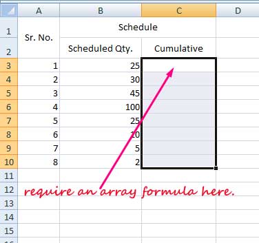
In my example, the data is in cells B3:B10, and I want to create a running total array formula in C3 to display the cumulative sum in C3:C10.

To implement this, a helper column (column A) is necessary, containing sequential numbers. In cell A3, enter the formula =ROW(B1:B8), then select A3:A10 and press Ctrl+Shift+Enter for Excel versions lacking dynamic array support.
Now, the final formula in cell C3 is =SUMIF(A3:A10, "<="&ROW(B1:B8), B3:B10). Enter this formula in C3, select C3:C10, and press Ctrl+Shift+Enter to generate expanding results in older Excel versions.
Formula Explanation:
Syntax: SUMIF(range, criteria, [sum_range])
It adds up values based on a specified condition.
In the formula:
range: A3:A10 – This is the cell range containing sequential numbers, acting as a helper column.criteria:"<="&ROW(B1:B8)– This is the condition for the SUMIF function. It checks if the sequential numbers in therangeare less than or equal to the current row sequential number.sum_range: B3:B10 – This range of values is undergoing calculation for the running total.
Running Total Array Formula Using MMULT in Excel
MMULT provides the flexibility to generate a cumulative sum in Excel without the need for a helper column.
By utilizing MMULT with the ROW function, you can calculate the cumulative sum, highlighting the crucial role played by the ROW function in both the SUMIF and MMULT solutions.
To implement this, enter the following running total array formula in cell C3:
=MMULT(IF(ROW(B3:B10)>=TRANSPOSE(ROW(B3:B10))=TRUE, 1, 0), B3:B10)After entering the formula in C3, select the range C3:C10 and press Ctrl+Shift+Enter to expand the result.
Note: If you encounter an error, blank cells within the range might be the cause. Ensure that you fill any blank cells with the value 0 to address this issue.
Formula Explanation:
Syntax: MMULT(array1, array2)
In the formula:
array1:IF(ROW(B3:B10)>=TRANSPOSE(ROW(B3:B10))=TRUE, 1, 0)– Creates a matrix of 1s and 0s. It checks if the row number in column B (from B3 to B10) is greater than or equal to the transposed row number (columns become rows and vice versa). If true, it assigns a value of 1; otherwise, it assigns 0.array2: B3:B10
This formula performs matrix multiplication (MMULT) of array1 with the values in the range B3:B10 (array2). The resulting array represents the cumulative sum for each corresponding row.
Running Total Using Dynamic Array in Excel
Users simplify running total calculations using the SCAN function in the latest versions of Excel.
Here’s the running total array formula using SCAN in Excel:
=SCAN(0, B3:B10, LAMBDA(a, v, a+v))Formula Explanation:
Syntax: =SCAN([initial_value], array, lambda(accumulator, value, formula_expression))
The SCAN function serves as a dedicated tool for calculating running totals in Excel, particularly in Microsoft 365.
initial_value: 0 – This is the initial value set in the accumulator and is defined asa.array: B3:B10 – the array to be scanned, with each element in the array defined asv.accumulator:avalue:vformula_expression:a+v
In each row, the SCAN formula systematically returns the intermediate calculation, resulting in a dynamic and evolving running total in Excel.
Conclusion
In summary, we explored three array formulas for running total calculations in Excel. The first two formulas are tailored for older versions of Excel, employing legacy CSE array formulas.
The third formula is designed for the latest versions of Excel, which support dynamic arrays, providing a more modern and efficient approach to running total calculations.


