You have two groups of 20 students each. How do you determine the rank of all students within their respective groups? We can use the COUNTIFS function to calculate the rank per group in Excel.

Rank per Group Using a Regular Formula

=COUNTIFS(group_range, current_group, score_range, ">" & current_score) + 1

Rank per Group Using a Dynamic Array Formula

=COUNTIFS(group_range, group_range, score_range, ">" & score_range) + 1

Overall Ranking

The sample data consists of names in column A, groups in column B, and scores in column C. To find the overall rank, enter the following formula in cell D2:

=RANK(C2, $C$2:$C$21)

and drag the fill handle (the blue square at the bottom of the active cell) down.

If you are using an Excel version that supports dynamic arrays, you can enter the following formula in cell D2, which will automatically expand down:

=RANK(C2:C21, C2:C21)

Examples of Group-wise Ranking in Excel

To determine the rank of students within their respective groups, known as group-wise ranking, you can use either the drag-down formula or a dynamic array formula.

Since the RANK function does not support conditional ranking in Excel, we use COUNTIFS as follows:

=COUNTIFS($B$2:$B$21, B2, $C$2:$C$21, ">"&C2) + 1

Enter this formula in cell E2 and drag the fill handle down.

Alternatively, if your version of Excel supports dynamic arrays, you can use this formula:

=COUNTIFS(B2:B21, B2:B21, C2:C21, ">"&C2:C21) + 1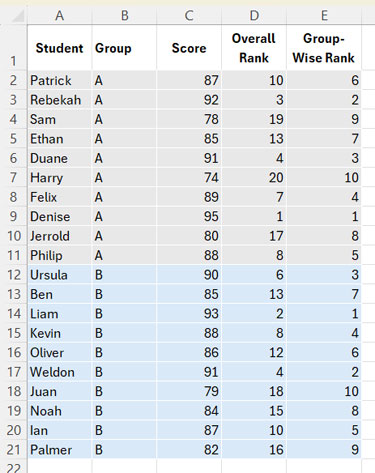

How Does COUNTIFS Return Rank per Group in Excel?

The COUNTIFS function is a conditional count function that accepts multiple conditions.

The formula:

=COUNTIFS($B$2:$B$21, B2, $C$2:$C$21, ">"&C2)

counts how many values within the same group (column B) have a higher score (column C) than the current row’s score.

• If the result is 0, adding +1 ensures the student receives the top rank.
• If the result is 1, adding +1 ensures the student receives the second rank, and so on.

When dragged down, this formula applies group-wise ranking to all scores in the range.

The dynamic array formula works the same way but without the need to drag it down manually.

That’s all about rank per group in Excel!

Resources

• Get Top N Values Using Excel’s FILTER Function
• Filter Top N per Category in Excel (Using FILTER & COUNTIFS)