")


")


")

")
")
 in Excel & Google Sheets")


If you’ve ever wanted Excel to automatically fill in a calendar with events from a table — you’re in the right place. In this tutorial, you’ll learn how to populate an Excel calendar dynamically using formulas only (no macros!).
By the end, you’ll have a calendar that updates instantly when you change the month or year, pulling events directly from your data table — perfect for project planning, deadlines, or team schedules.
Why Create a Dynamic Calendar in Excel?
Before diving into formulas, let’s understand why this approach matters. A dynamic calendar is not just a grid of numbers — it’s a living schedule that responds to your data.
Unlike static tables, it:
- Adjusts automatically for any month or year
- Pulls event data directly from your table
- Visually highlights today and the current week
- Works perfectly for planning or reporting dashboards
Now that you know the “why,” let’s roll up our sleeves and build one.
Let’s first set up the calendar layout — the foundation for everything that follows.
Along the way, we’ll also add a few clever conditional formatting tricks to keep the calendar clean and highlight only the right date cells.
Step 1: Build the Dynamic Calendar Framework
To populate an Excel calendar automatically, we first need a calendar structure that can react to user input. We’ll start by creating drop-down controls for month and year, then generate the calendar grid dynamically.
1.1 Add Month and Year Controls
- In B1, type
Select Month. - In C1, type
Enter Year. - Select B2, then go to Data → Data Validation → List.
- Paste this in the Source field:
January,February,March,April,May,June,July,August,September,October,November,December - Click OK. You now have a clean drop-down for month selection.

In B2, select any month — for example, October — and in C2, type any year, such as 2025. These cells will control which month and year your calendar displays.
1.2 Add Weekday Names
With the month and year ready, it’s time to build the calendar layout.
In B4:H4, type weekday names from Sunday through Saturday.
1.3 Generate the Calendar Grid with a Formula
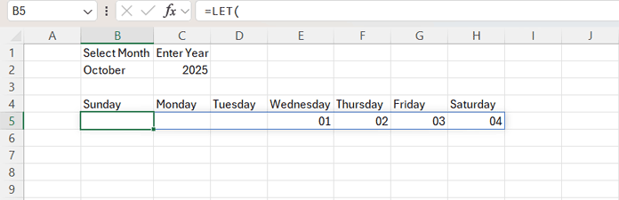
To generate the first row of your dynamic calendar, enter the following formula in B5:
=LET(
  my, DATE(C2, MONTH(B2&1), 1),
  dts, SEQUENCE(1, 7, my-WEEKDAY(my)+1),
  fnl, dts*(EOMONTH(dts, 0)=EOMONTH(my, 0)),
  IF(fnl, fnl, "")
)
Then, select the range B5:H5, navigate to Home → Format → Format Cells, choose Custom, type DD under Type, and click OK. This formats the cells to display only the day portion of each date.
This clever formula:
- my – identifies the first day of the selected month and year.
- dts – creates a sequence of seven dates, representing one week, starting from the Sunday (or your first weekday) of that month.
- fnl – checks whether each date in the sequence belongs to the same month as the selected one and replaces dates outside that month with blank cells.
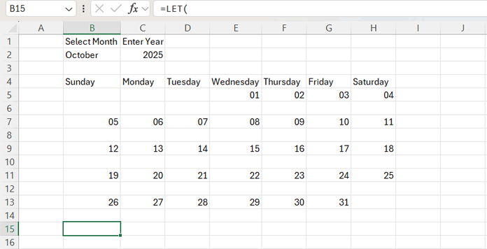
To extend it, in B7, enter this next formula:
=LET(
  my, DATE($C$2, MONTH($B$2&1), 1),
  dts, SEQUENCE(1, 7, H5+1),
  fnl, dts*(EOMONTH(dts, 0)=EOMONTH(my, 0)),
  IFERROR(IF(fnl, fnl, ""), "")
)
Copy it from cell B7 down to B9, B11, B13, and B15, and format those rows to DD as mentioned earlier.
The formula works as follows:
my— calculates the first date of the selected month and year.dts— generates a sequence of 7 dates starting from the day after the last date of the previous row (H5+1).fnl— ensures only dates within the selected month are displayed; dates outside the month return 0.IFERROR(IF(fnl, fnl, ""), "")— replaces any zero or error values with a blank, keeping the calendar grid clean.
Now your calendar changes dynamically as you adjust the month or year.
With the framework ready, it’s time to bring it to life with event data.
Step 2: Populate the Dynamic Excel Calendar from a Data Table
The calendar grid is ready, but it’s still empty. Let’s make it meaningful by pulling events from a structured data table.
2.1 Create the Event Data Table
Add a new sheet and name it Event Data.
Note: You can add a new sheet by clicking the plus (+) button at the bottom. To rename a sheet, double-click the tab name. You can also rename the dynamic calendar sheet to “Calendar View.”
In B3:E3, create the following headers:
- Date
- Event Title / Description
- Category
- Status
Fill in some sample events like this:
| Date | Event Title / Description | Category | Status |
|---|---|---|---|
| 04-10-2025 | Report Due | Deadline | In Progress |
| 05-10-2025 | Phase 1 Complete | Milestone | Completed |
| 07-10-2025 | Client Call | Meeting | Scheduled |
| 18-10-2025 | Launch Day | Milestone | Scheduled |
Select the range and go to Insert → Table. In the dialog box, check “My table has headers” and click OK.
Go to any cell within the table and click on Table Design. Under Table Name, enter Event_Data.

This is your event list table — the heart of your dynamic calendar.
2.2 Link Events to the Calendar Grid
Now we’ll connect your table to the calendar.
Go back to the Calendar sheet, and in B6, enter:
=IFERROR(
  TEXTJOIN(
    CHAR(10),
    TRUE,
    FILTER(Event_Data[Event Title / Description], ((Event_Data[Date]> 0)*(Event_Data[Date]=B5)))
  ), ""
)
This formula filters the Event Title / Description column in the Event_Data table for rows where the date matches B5, then joins the results with a new line character.
Next, select B6 and click Wrap Text in the Home tab under the Alignment group.
Copy this formula from B6 across C6:H6, then down to B8:H8, B10:H10, B12:H12, B14:H14, and B16:H16. Each date will now display events that match its date automatically.
Select rows 5 to 16 and double-click the row numbers to auto-adjust row height and see all the text.
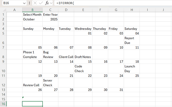
Your Excel calendar is now alive! Next, we’ll make it visually appealing with some formatting.
Step 3: Add Smart Conditional Formatting
You’ve got a functional calendar — now let’s make it visually intuitive.
We’ll use conditional formatting to highlight today, show the current week, and define clear borders.
Select the range B5:H16, then go to:
Home → Conditional Formatting → New Rule → Use a formula to determine which cells to format
Add these conditional formatting rules:
| Purpose | Formula | Format |
|---|---|---|
| Add borders (dates & events) | =IFERROR(YEAR(B5)=$C$2,"") | Bold dark-blue font, borders: top, left, right |
| Add borders (dates & events) | =IFERROR(YEAR(B4)=$C$2,"") | Borders: bottom, left, right |
| Highlight current week | =OR(IFERROR(WEEKNUM(B4), "")=WEEKNUM(TODAY()), IFERROR(WEEKNUM(B5), "")=WEEKNUM(TODAY())) | Light blue background |
| Highlight today | =OR(B5=TODAY(), B4=TODAY()) | Green background, white text |
Click View and uncheck Gridlines, then adjust the column and row widths as desired. With these final touches, your calendar will look polished and dynamic.
FAQs
How do I change the week layout to Monday–Sunday?
Change weekday labels in B4:H4 to Monday–Sunday.
In the B5 formula, replace:
WEEKDAY(my)+1with:
WEEKDAY(my, 2)+1Then adjust your “current week” conditional formatting rule to use WEEKNUM(..., 2).
Which Excel versions support this dynamic calendar?
This setup requires Excel 365 or Excel 2021, which support the LET, SEQUENCE, and FILTER functions.
Final Thoughts
And there you have it — a fully automated, formula-driven dynamic Excel calendar that populates itself from your event table.
What started as a simple grid is now a smart planner — capable of showing today’s date, highlighting your current week, and displaying upcoming events at a glance.
Once you try it, you’ll wonder how you ever managed your schedules without it.
Get the ready-to-use Excel Dynamic Calendar file:
Want to take your calendar to the next level?
Check out my latest tutorial — Create a Smart Excel Calendar with Task Durations — to build a version that handles multi-day tasks, status filters, and automatic highlights without using VBA.
The formula does not seem to return all of the event descriptions for a given date. Does something need to be adjusted to allow more than three to populate?
It may be hidden within the cell. Try increasing the row height. Instead of double-clicking the row number, drag the row number separator downward to reveal the remaining content.
Unfortunately, that did not help. I have also noticed that some of the “Events” are not showing. Any other thoughts?
It works correctly on my end. If some events are missing, it’s usually due to data issues (dates containing time values or dates stored as text). Since I can’t review Excel files here, please double-check the source data.
QUESTION – Using the example you have outlined above, if I want to have the calendar filtered by the column Category, what would the formula look like? How would it change from this:
=IFERROR(TEXTJOIN(
CHAR(10),
TRUE,
FILTER(Event_Data[Event Title / Description], ((Event_Data[Date]> 0)*(Event_Data[Date]=B5)))
), ""
)
You can use the formula as follows:
=IFERROR(TEXTJOIN(
CHAR(10),
TRUE,
FILTER(
Event_Data[Event Title / Description],
((Event_Data[Date]>0)*(Event_Data[Date]=B5)*(Event_Data[Category]="Meeting"))
)
),
""
)