


")


")


Marking case-sensitive unique values provides several benefits compared to merely extracting them in an Excel spreadsheet.
I’m referring to a formula that returns TRUE if a value is case-sensitively unique; otherwise, it returns FALSE. Once you achieve this, you can use these Boolean values for numerous tasks in Excel, such as:
- Extracting case-sensitive unique values in a column
- Filtering case-sensitive unique records
- Highlighting duplicates based on case sensitivity
We do not rely on any drag-down formulas for this. To mark case-sensitive unique values, you can use the following formula in Excel:
=VSTACK(TRUE,MAP(A1:A7, A2:A8, LAMBDA(value1,value2,NOT(OR(EXACT(A1:value1,value2))))))Example of Marking Case-Sensitive Unique Values in Excel
Consider an Excel spreadsheet with some values in the range A1:A8. If you apply the above formula in B1, the result will be as follows:
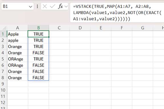
This method effectively marks case-sensitive unique values in an Excel spreadsheet.
How to Adapt the Formula
When using this formula, make these adjustments:
- Replace
A1with the cell reference of the first row in the range. - Replace
A1:A7with the range reference from the first row to the second-to-last row. - Replace
A2:A8with the range reference from the second row to the last row.
Formula Explanation
=VSTACK(TRUE,MAP(A1:A7, A2:A8, LAMBDA(value1,value2,NOT(OR(EXACT(A1:value1,value2))))))The EXACT(A1:value1, value2) function compares values case-sensitively. The MAP function iterates through each value in the arrays, so the formula processes pairs like EXACT(A1:A1, A2), EXACT(A1:A2, A3), and EXACT(A1:A3, A4).
The EXACT function returns an array of TRUE or FALSE values. If the current row value appears anywhere above, the EXACT output will include a TRUE.
The OR function combines the results of EXACT to determine if a match exists.
The NOT function converts TRUE to FALSE, ensuring that unique values return TRUE. If a value appears anywhere above, the formula will mark it as FALSE.
This process corresponds to rows 2 through the last row in the range. The first row will always be considered a unique value, so we append a TRUE at the top using VSTACK.
Real-Life Uses of Marking Case-Sensitive Unique Values in Excel
As mentioned earlier, marking rows containing case-sensitive unique values has several benefits:
1. Extract Case-Sensitive Unique Values
To extract case-sensitive unique values from a range, use:
=FILTER(A1:A8, B1#)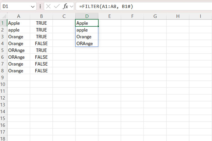
If you prefer not to use the helper formula in B1, replace B1# with the MAP formula directly.
2. Filter Records from Case-Sensitive Unique Rows
Follow a similar approach to filter case-sensitive unique records in a table. Mark the relevant column using the formula and filter the table based on the Boolean results.
3. Highlight Case-Sensitive Unique Values
To highlight case-sensitive unique values:
- Select the range
A2:A8. - Click Home > Conditional Formatting > New Rule.
- Select “Use a formula to determine which cells to format.”
- Enter:
=B1=TRUE - Click Format and choose a fill color.
- Click OK to close the Format Cells dialog box.
- Click OK to close the New Formatting Rule dialog box.
This will highlight the case-sensitive unique values in the selected range.