


")


")

")
")
 in Excel & Google Sheets")


In a large vertical dataset in Excel, how do you find the cell address of the last value in the last used row?
Assume the data range is A1:Z1000, and the last used row is row 250. In that row, the last value appears in column E. Therefore, the last used row’s last value address is E250.
You can dynamically find this in Excel using modern functions such as TRIMRANGE, XLOOKUP, and REGEXREPLACE.
Formula to Find the Last Used Row’s Last Value Address in Excel
=LET(range, "A1:Z1000", lur, MAX(ROW(TRIMRANGE(INDIRECT(range), 3, 3))), cr, REGEXREPLACE(range,"\d+", lur), val, XLOOKUP(TRUE, INDIRECT(cr)<>"", INDIRECT(cr), "", 0, -1), CELL("address", val))Replace "A1:Z1000" with the actual range you want to check.
Where Does This Formula Come in Use?
When working with large datasets, knowing the last used row’s last value address can be useful in many ways:
- Use it with INDIRECT, INDEX, HYPERLINK, or Conditional Formatting to navigate, highlight, or extract data dynamically.
- Create dynamic ranges that expand automatically as new data is added.
Since our focus is on extracting the cell address rather than just the row number, let’s see a real-life example.
Example
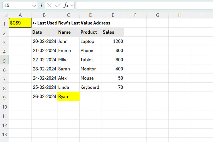
Consider the following dataset in B2:E9, which grows over time. For flexibility, we define the range as B2:E10000.
Using the formula:
=LET(range, "B2:E10000", lur, MAX(ROW(TRIMRANGE(INDIRECT(range), 3, 3))), cr, REGEXREPLACE(range, "\d+", lur), val, XLOOKUP(TRUE, INDIRECT(cr)<>"", INDIRECT(cr), "", 0, -1), CELL("address", val))At present, this formula returns C9.
If you scroll to row 110 and enter any value, say “X” in E110, the formula will update and return E110.
Things to Know
- Enter the formula outside the specified range to avoid errors.
- If your data is on Sheet1 and you use the formula from another sheet, modify it as follows:
=LET(range, "B2:E10000", lur, MAX(ROW(TRIMRANGE(INDIRECT("Sheet1!"&range), 3, 3))), cr, REGEXREPLACE(range, "\d+", lur), val, XLOOKUP(TRUE, INDIRECT("Sheet1!"&cr)<>"", INDIRECT("Sheet1!"&cr), "", 0, -1), CELL("address", val))This will return the cell address with the sheet and file name, e.g.:
'[Sales Data.xlsx]Sheet1'!$E$110
Here, 'Sales Data.xlsx' is the file name, and Sheet1!$E$110 is the cell address.
How the Formula Works
The formula is built using LET to break it into components:
range:"B2:E10000"→ Defines the dataset.lur:MAX(ROW(TRIMRANGE(INDIRECT(range), 3, 3)))→ Finds the last used row number (see: Find the Last Used Row Number in Excel).cr:REGEXREPLACE(range, "\d+", lur)→ Replaces row numbers in therangewithlur(last used row number).val:XLOOKUP(TRUE, INDIRECT(cr)<>"", INDIRECT(cr), "", 0,- 1)→ Identifies the last non-empty value in that row.CELL("address", val)→ Returns the cell address of the last value.
Related Resources
- Hyperlink to Jump to the Last Used Row in Excel
- Find the Last Column with Data in Excel (Not Just Column Count)
- Highlight the Last Used Row in Excel