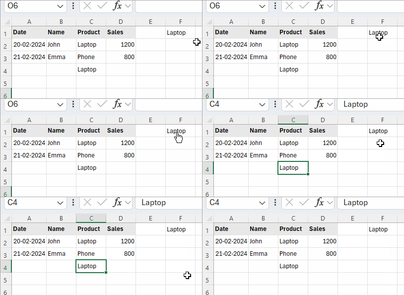
Hyperlink to Jump to the Last Used Row in Excel

In a vertical range, you can create a hyperlink to jump to the last used row in Excel. The formula not only fetches the last used value but also links to it. This allows you to place a clickable link at the top of your spreadsheet, enabling quick navigation to the last used cell.

Formula to Create a Hyperlink to the Last Used Row

Use the following formula:

=LET(range, "A1:Z1000", lur, MAX(ROW(TRIMRANGE(INDIRECT(range), 3, 3))), cr, REGEXREPLACE(range, "\d+", lur), val, XLOOKUP(TRUE, INDIRECT("Sheet1!"&cr)<>"", INDIRECT("Sheet1!"&cr), "", 0, -1), HYPERLINK("#"&CELL("address", val), val))

How to Use:

Replace A1:Z1000 with your actual data range.
Replace Sheet1 with the name of the sheet containing the data.
Ensure the formula is placed outside the specified range.

Important Notes:

Avoid open-ended ranges like A:Z, as the formula does not support them. Instead, define a fixed range (e.g., A1:Z1000) that accommodates both existing and future data.

Example: Creating a Hyperlink to the Last Used Row in Excel

Assume your data is in columns A to D, and the last used row is currently row 4, with the last value in cell C4. To create a hyperlink in cell F1, use this formula:

=LET(range,"A1:D1000",lur,MAX(ROW(TRIMRANGE(INDIRECT(range),3,3))),cr,REGEXREPLACE(range,"\d+",lur),val,XLOOKUP(TRUE,INDIRECT("Sheet1!"&cr)<>"",INDIRECT("Sheet1!"&cr),"",0,-1),HYPERLINK("#"&CELL("address",val),val))

Since the last used value is “Laptop” in C4, the formula will return that value as a clickable hyperlink in F1.

Hyperlink to the last used row's last value in Excel

Clicking the hyperlink will take you directly to cell C4.

Testing the Formula:

Enter any new value in columns A, B, or C.
Example: If you enter "Test" in cell C100, the hyperlink in F1 will update to "Test", linking to C100.

Frequently Asked Questions

Can I use this formula to jump to the last used row in another sheet within the same workbook?

Yes, as long as you correctly specify the sheet name in the formula.

How does this formula work?

This formula builds upon previous methods for finding the last used row in Excel but modifies them to create a hyperlink.

Breakdown of the formula:

range
"A1:D1000" – The defined range in which you want to create the hyperlink.
lur (Last Used Row)
MAX(ROW(TRIMRANGE(INDIRECT(range), 3, 3))) – Finds the last used row number.
cr (Cell Reference)
REGEXREPLACE(range, "\d+", lur) – Constructs the row address for the last used row.
val (Last Used Value)
XLOOKUP(TRUE, INDIRECT("Sheet1!"&cr)<>"", INDIRECT("Sheet1!"&cr), "", 0, -1) – Retrieves the last used value.
Hyperlink Creation
HYPERLINK("#"&CELL("address", val), val) – Generates a hyperlink pointing to the last used row.

What is the logic behind this formula?

TRIMRANGE trims the range and ROW returns row numbers.
MAX identifies the highest row number (i.e., the last used row).
REGEXREPLACE updates the range reference to point to this row.
XLOOKUP retrieves the last used value in that row.
The HYPERLINK function then makes the value clickable.

Additional FAQs

Does this formula work in all versions of Excel?

No, this formula requires Excel 365 or a supported version, as it relies on functions like LET, TRIMRANGE, and REGEXREPLACE.

Can I use an open-ended range (e.g., A:Z)?

No, the formula is designed for closed ranges to ensure accuracy.

Can I hyperlink to the last used row in another sheet?

Yes, simply specify the correct sheet name in the formula.

Summary

With this formula, you can create a hyperlink to jump to the last used row in Excel, making data navigation more efficient. Simply place the formula in a cell outside your data range, and it will dynamically update as new data is entered.

Let me know if you have any questions!