")
")


")


")

")
")
 in Excel & Google Sheets")


When using the FILTER function in Excel to extract the top N values, it’s important to account for duplicates in the amount column.
In this tutorial, you will learn how to obtain top entries using FILTER and other Excel functions.
FILTER is a component of dynamic array functions in Excel, available in Microsoft 365 and Excel 2021.
Sample Data and Filtering Objective
We have a sample sales dataset in an Excel spreadsheet, containing columns for names, departments, sales amounts, and regions spanning cells A1 to D21. The labels Name, Department, Sales, and Region are in cells A1 to D1, respectively.
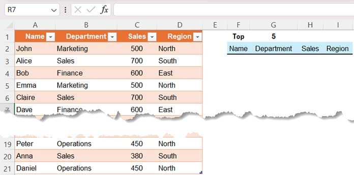
Our task is to identify the top 3, 5, 10, 20, or ‘n’ sales figures from all regions or a specified region. If we enter ‘5’ in cell G1, a formula in cell F3 should extract the top 5 sales value entries from A1:D21. How can we achieve this in Excel?
Additionally, if the sales amount column contains duplicates, how should we address them?
1. Unique Top N + All Occurence of these Values
In this approach, the formula will filter the unique top N values, and if any of these values occur more than once, all of their occurrences will be included.
Step 1: Determining Maximum Unique Entries in the Amount Column
This step is crucial. While you may have numerous rows of data, if the amount column (the max column) contains only 10 unique entries, specifying ’20’ in cell G1 to filter the top 20 entries will result in a formula failure.
To prevent this, it’s advisable to ascertain the total number of unique values before filtering the top ‘n’ values.
Enter the following formula in any blank cell:
=COUNT(UNIQUE(C2:C21))If it returns ‘8’, you can enter any number between 1 and 8 in cell G1.
The above formula provides the maximum number of unique records concerning sales that can be filtered from the range A1:D21.
Step 2: Using the FILTER Function to Extract Top N Values in Excel
Let me provide you with the generic formula, so you can easily adapt it to your data. Then we will apply the same to our sample dataset.
Generic Formula:
=SORT(FILTER(range, amount_column>=LARGE(UNIQUE(amount_column), n)), amount_column_index, -1)So the formula in cell F3 for our sample dataset will be:
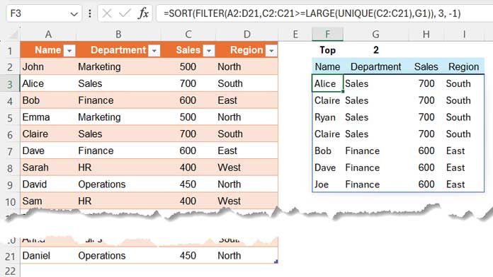
=SORT(FILTER(A2:D21, C2:C21>=LARGE(UNIQUE(C2:C21), G1)), 3, -1)In this formula, the value in cell G1 is 5. If you enter 3 in cell G1, the formula will return the top 3 values.
Formula Breakdown:
FILTER(A2:D21, C2:C21>=LARGE(UNIQUE(C2:C21), G1)) – filters the range A2:D21 based on the condition C2:C21>=LARGE(UNIQUE(C2:C21), G1).
In the condition, the UNIQUE function returns the unique amounts in column C (C2:C21), and the LARGE function returns the nth largest value from these unique amounts.
The FILTER function filters the range if the value in the amount column (C2:C21) is greater than or equal to the nth largest value in the amount column.
The SORT function sorts the filtered range in descending order based on the amount column to arrange the largest amounts at the top.
Does the Formula Account for Duplicate Amounts?
Yes, it does! If the sales amounts are {20, 20, 5, 5, 1, 1}, the top 2 will include {20, 20, 5, 5}, not just {20, 20}.
Please refer to this screenshot for clarification.
How to Extract Unique Top N Values Based on a Condition in Excel
Suppose you want to retrieve the top ‘n’ sales values from the North region. You can achieve this by incorporating an additional condition within the FILTER function, i.e., (D2:D21="North"), and applying a filtered range within the UNIQUE function.
Generic Formula:
=SORT(FILTER(range, (criteria_column=criteria)*(amount_column>=LARGE(UNIQUE(FILTER(amount_column, criteria_coulmn=criteria)), n))), amount_column_index, -1)Formula:
=SORT(FILTER(A2:D21, (D2:D21="North")*(C2:C21>=LARGE(UNIQUE(FILTER(C2:C21, D2:D21="North")), G1))), 3, -1)Where:
A2:D21: Range to filter(D2:D21="North"): Filter condition 1(C2:C21>=LARGE(UNIQUE(FILTER(C2:C21, D2:D21="North")), G1)): Filter condition 2
The asterisk is an alternative to AND, signifying that both conditions must be TRUE.
2. Filter Top N Values + All Occurrences of the Nth Value in Excel
In this approach, the formula will filter the top N values, and if the Nth value appears more than once, all its occurrences will be included.
Generic Formula:
=SORT(FILTER(range, RANK(amount_column, amount_column)<=n), amount_column_index, -1)How to apply it?
Step 1: Entering N in a Helper Cell
To filter the top 10 values, enter 10 in cell G1.
Note: If your data range contains fewer than 10 rows, entering 10 in G1 won’t break the formula. Instead, it will return all the available records.
Step 2: Applying the Formula
=SORT(FILTER(A2:D21, RANK(C2:C21, C2:C21)<=G1), 3, -1)- The FILTER function extracts data from A2:D21 where the rank of C2:C21 is less than or equal to the value in G1.
- The SORT function then arranges the results in descending order based on the specified column index.
How to Extract Top N Values + All Occurrences of the Nth Value Based on a Condition in Excel
Since the RANK function does not support conditions, we will use COUNTIFS instead.
Generic Formula:
=SORT(LET(rank, (COUNTIFS(criteria_column, criteria, amount_column, ">"&amount_column)+1)*(criteria_column=criteria), FILTER(range, (rank<=n)*(rank>0))), amount_column_index, -1)Example:
The following formula filters the top 3 (if G1 is 3) items from the North region:
=SORT(LET(rank, (COUNTIFS(D2:D21, "North", C2:C21, ">"&C2:C21)+1)*(D2:D21="North"), FILTER(A2:D21, (rank<=G1)*(rank>0))), 3, -1)- The COUNTIFS function calculates the rank of sales within the North region.
- The FILTER function extracts rows where the rank is within the top N.
- The SORT function arranges the results in descending order based on column index 3.