As you may know, Pivot Tables in Excel are case-insensitive by default. To create a case-sensitive Pivot Table in Excel, you need to use some workarounds.

The workaround involves three steps to be completed before creating the case-sensitive Pivot Table report:

1. Extract case-sensitive unique values
   Identify and extract unique values from the column you want to group, preserving case sensitivity.
2. Assign a sequence to the extracted values
   Generate a sequence for the extracted values while ignoring case sensitivity.
3. Create a helper column
   Use the assigned sequence to create a helper column. This helper column will replace the original column for grouping in the Pivot Table.

Sample Data for Creating a Case-Sensitive Pivot Table in Excel

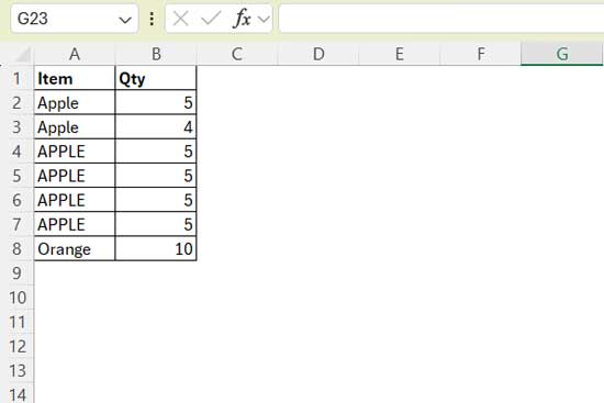
We will use the following sample data in A1:B for this purpose:

The goal is to create a Pivot Table report grouped by Item and return the total quantity. If you use a regular Pivot Table, the result would look like this:

• Apple: 29
• Orange: 10

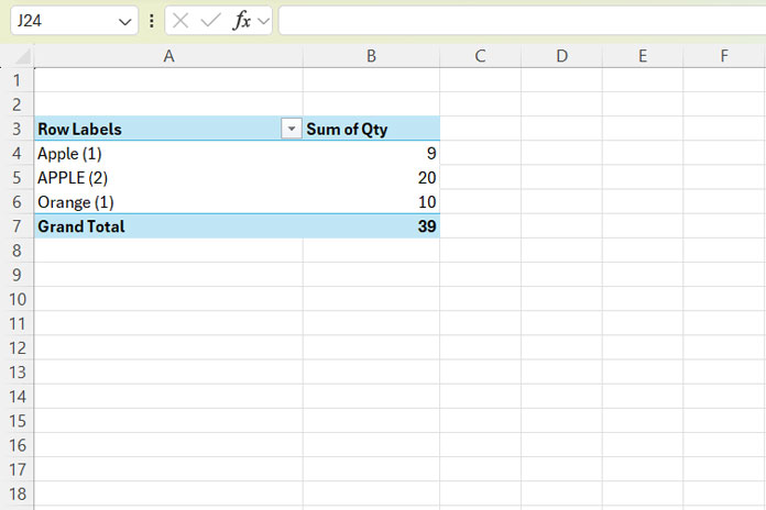
However, we want the output to reflect case sensitivity:

• Apple: 9
• APPLE: 20
• Orange: 10

Let’s see how to achieve that.

Creating the Helper Column for a Case-Sensitive Pivot Table in Excel

1. Extracting Case-Sensitive Unique Values from the Group Column

We want to extract unique values from column A while maintaining case sensitivity. Since the UNIQUE function in Excel is not case-sensitive, we will use the following formula:

=REDUCE(,A2:A8,LAMBDA(acc,val,IF(SUMPRODUCT(EXACT(acc,val)*1),acc,VSTACK(acc,val))))

Enter this formula in cell D2.

How the formula works:

• REDUCE processes the array A2:A8 iteratively, applying a LAMBDA function to each element.
• The LAMBDA function is:IF(SUMPRODUCT(EXACT(acc,val)*1),acc,VSTACK(acc,val))
  • acc: Stores intermediate results (starts as an empty array).
  • val: Refers to the current element in the array.
  • EXACT(acc,val): Checks if the current element matches any element in acc (case-sensitive).
  • If no match is found, VSTACK adds val to acc; otherwise, acc remains unchanged.

2. Assigning a Sequence to the Extracted Values

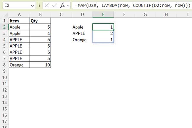
In cell E2, enter the following formula:

=MAP(D2#, LAMBDA(row, COUNTIF(D2:row, row)))

This returns a running count of the case-sensitive unique values extracted in the previous step.

Related: Running Count of Occurrences in Excel (Includes Dynamic Array)

3. Creating the Helper Column for the Case-Sensitive Pivot Table

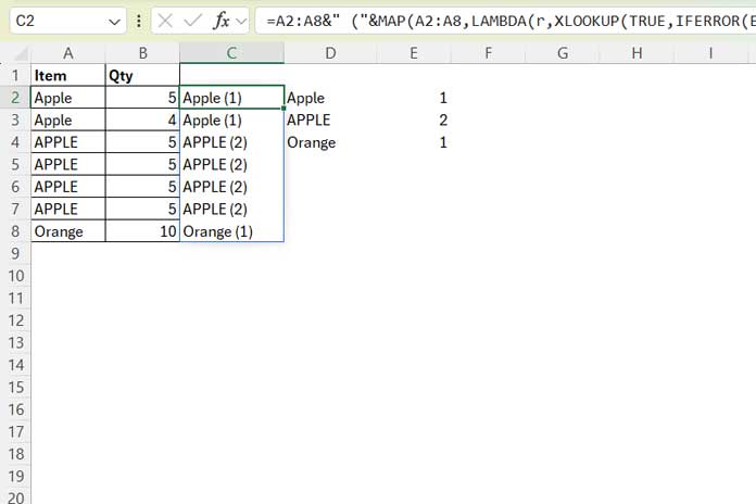
Next, we will assign the values in the group column with their corresponding sequence. Use the following formula in cell C2:

=A2:A8&" ("&MAP(A2:A8,LAMBDA(r,XLOOKUP(TRUE,IFERROR(EXACT(r,D2#),""),E2#)))&")"

Explanation:

• This formula searches for values in A2:A8 within D2# and returns the corresponding value from E2#. The search is case-sensitive because of the combination of EXACT and XLOOKUP.
• Each occurrence of “Apple” becomes “Apple (1)”, while “APPLE” becomes “APPLE (2)”, and so on.
• Adding a number to each value ensures that Excel treats them as distinct entries in the Pivot Table.

Related: How to Perform Case-Sensitive XLOOKUP in Excel with EXACT

4. Labeling the Helper Column

Enter a header, such as Item, in cell C1 for the helper column.

Creating the Case-Sensitive Pivot Table in Excel

Follow these steps to create the Pivot Table:

1. Select the range B1:C8, excluding the original group column A but including the helper column C.
2. Go to the Insert tab in Excel and click Pivot Table in the Tables group.
3. In the dialog box that appears, click OK.
4. A new worksheet will open with the Pivot Table layout.
5. In the Pivot Table Fields pane, check Item and Qty.

The resulting Pivot Table will display the data grouped case-sensitively:

Resources

• Unpivot Excel Data Fast: Power Query & Dynamic Array Formula
• Case-Sensitive Pivot Table in Google Sheets
• Marking Case-Sensitive Unique Values in Excel