This tutorial explains how to create a calendar in Excel using a one-line formula that utilizes dynamic array functions.

I call it the most efficient method to create a calendar in Excel as it showcases how to create a sequence of dates and arrange them under the proper weekday names using the correct functions.

The formula returns each month’s calendar corresponding to the month selected in one cell and the year entered in another cell.

Alternatively, you can create a full-year calendar with just one modification to the monthly formula.

Step 1: Create a Drop-Down Menu for Month Selection

1. Navigate to cell A1.
2. Click on “Data Validation” in the “Data Tools” group under the “Data” menu.
3. Select “List” from the “Allow” drop-down menu.
4. In the “Source” field, enter the month names January to December separated by commas or copy-paste this: Jan, Feb, Mar, Apr, May, Jun, Jul, Aug, Sep, Oct, Nov, Dec.
5. Click OK.

This will create a drop-down list for month selection. Please select any month, for example, “Mar”.

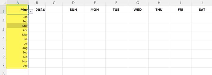
Step 2: Enter the Year and Weekday Names in a Row

In cell B1, enter any year, for example, 2024.

Then, enter the weekday names Sunday to Saturday in cells D1 to J1. Please refer to the image above.

This step is independent of the one-line formula that creates the monthly calendar, so you can enter weekday names in full or abbreviated form.

You are free to choose any location to enter the weekday names, as we only need to enter the one-line dynamic array formula in one cell, e.g., under Sunday, to generate the monthly or yearly calendar.

Step 3: Unformatted Calendar Formula.

We can indeed utilize the SEQUENCE function in Excel to generate an unformatted dynamic calendar in a row or column.

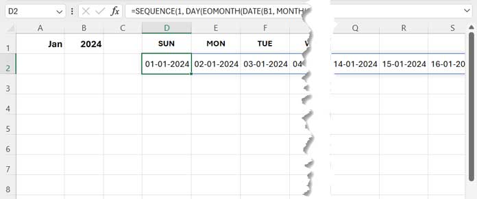
For example, the following code in cell D2 will generate a sequence of dates for January 2024 in a row (assuming January is selected in cell A1 and 2024 is entered in cell B1):

=SEQUENCE(1, DAY(EOMONTH(DATE(B1, MONTH(A1&1), 1),0)),  DATE(B1, MONTH(A1&1), 1))

This dynamic array formula adheres to the syntax: =SEQUENCE(rows, columns, start)

• rows: 1
  We presently need the dates in one row.
• columns: DAY(EOMONTH(DATE(B1, MONTH(A1&1), 1),0))
  We need the sequence in ‘n’ number of columns where ‘n’ is the number of days in the month. We have used the month selected in cell A1 and the year entered in cell B1 to create the month’s start date, i.e., DATE(B1, MONTH(A1&1), 1). If you want to learn more about this formula, please check out: Excel: Month Name to Number & Number to Name.
  We have converted this date to the end of the month using EOMONTH.
  The DAY function returns the day part, which is the number of days in the selected month and entered year in A1 and B1, respectively.
• start: We need the sequence to start at DATE(B1, MONTH(A1&1), 1).

The result will be date values. You should select the result and then choose “Short Date” within the “Number” group under the “Home” tab.

Step 4: Offsetting Columns to Align the Start Date with the Correct Weekday

One challenge in creating a dynamic calendar in an Excel spreadsheet is arranging the dates under the correct weekday names by offsetting columns.

In the example above, the weekday name of 01-01-2024 is Monday. Currently, this date is placed under Sunday as the formula starts in cell D2.

If you select a different month, for example, February, the formula will return the date 01-02-2024 in D2, which will be a Thursday.

How can we ensure the month’s starting date is placed in an Excel calendar under the correct weekday column?

This is where the one-line formula works its magic to create the calendar.

To place the dates under the correct weekday names, we need to horizontally stack ‘n’ blank cells with the dates, where ‘n’ will be the weekday number of the starting date of the month. For this purpose, we can use the EXPAND function.

Related: EXPAND + Stacking: Expand an Array in Excel

The following formula expands the array, which is an empty value, based on the weekday number of the month’s start date. If it’s Sunday, it will expand by 1 column, for Monday 2 columns, and so on.

=EXPAND("",,WEEKDAY(DATE(B1, MONTH(A1&1), 1)))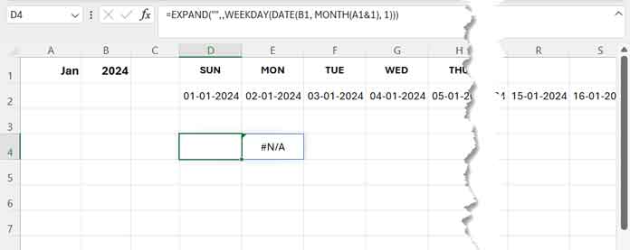

It adheres to the following syntax: =EXPAND(array, , columns), where columns is the weekday number.

In the expanded columns, the formula will return #N/A values. We will remove those later.

We should horizontally stack this output with the sequence formula from Step #3.

=HSTACK(EXPAND("",,WEEKDAY(DATE(B1, MONTH(A1&1), 1))), SEQUENCE(1, DAY(EOMONTH(DATE(B1, MONTH(A1&1), 1),0)), DATE(B1, MONTH(A1&1), 1)))

Then remove one empty cell using the DROP function.

=DROP(HSTACK(EXPAND("",,WEEKDAY(DATE(B1, MONTH(A1&1), 1))), SEQUENCE(1, DAY(EOMONTH(DATE(B1, MONTH(A1&1), 1),0)), DATE(B1, MONTH(A1&1), 1))),,1)

This follows the syntax: =DROP(array, , columns).

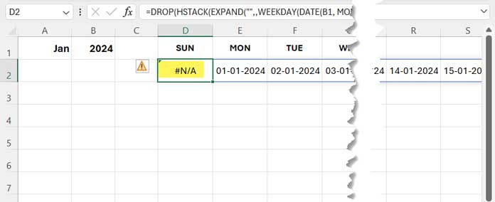
This aligns the start date with the correct weekday column.

Step 5: Wrapping Rows Based on 7 Values in a Row

We currently have a formula that returns a calendar based on the selected month and year. It correctly offsets columns based on the weekday of the month’s starting date.

We need to organize the result by allowing 7 values in each row. We will use the WRAPROWS function for that purpose.

=WRAPROWS(DROP(HSTACK(EXPAND("",,WEEKDAY(DATE(B1, MONTH(A1&1), 1))), SEQUENCE(1, DAY(EOMONTH(DATE(B1, MONTH(A1&1), 1),0)),  DATE(B1, MONTH(A1&1), 1))),,1), 7)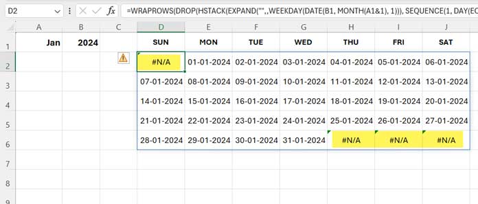

It follows the syntax: =WRAPROWS(vector, wrap_count), where vector is the result of the formula from Step 4 and wrap_count is 7.

Note: You should select the result range and format the values as dates (I’ve already explained how to do this above).

Step 6: Removing Error Values

Finally, wrap the formula with IFERROR to replace error values with blanks.

=IFERROR(WRAPROWS(DROP(HSTACK(EXPAND("",,WEEKDAY(DATE(B1, MONTH(A1&1), 1))), SEQUENCE(1, DAY(EOMONTH(DATE(B1, MONTH(A1&1), 1),0)), DATE(B1, MONTH(A1&1), 1))),,1), 7),"")

Step 7: Improving Performance

The formula currently calculates DATE(B1, MONTH(A1&1), 1) multiple times. We can use the LET function to name this formula expression as “dt” and use “dt” instead of DATE(B1, MONTH(A1&1), 1) in the subsequent formula to avoid repeated calculations. This will also enhance the readability of the formula.

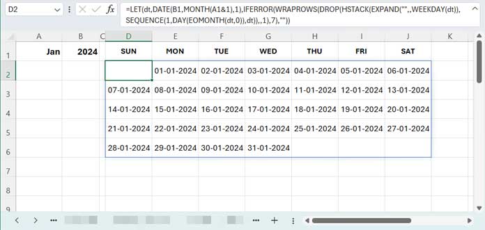
=LET(dt,DATE(B1,MONTH(A1&1),1),IFERROR(WRAPROWS(DROP(HSTACK(EXPAND("",,WEEKDAY(dt)),SEQUENCE(1,DAY(EOMONTH(dt,0)),dt)),,1),7),""))

Step 8: Converting to Full-Year Calendar

The above formula generates a monthly calendar in Excel that produces each month’s dates based on the month selected in cell A1.

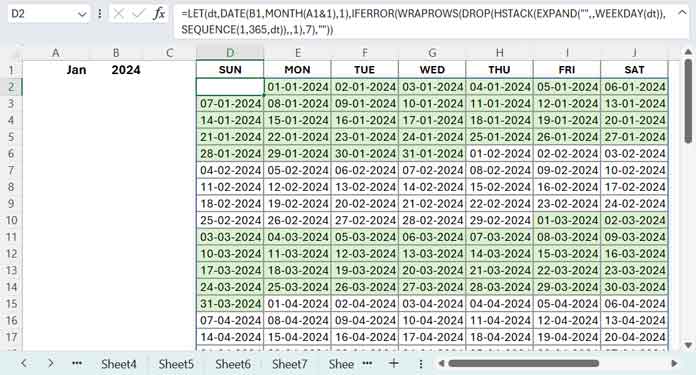
If you want a full-year calendar, select January in cell A1.

Then replace DAY(EOMONTH(dt, 0)) in the formula with either 365 or 366 depending on whether the year in cell B1 is a leap year or not. The rule of thumb is to use 365 if February has 28 days, and 366 if February has 29 days.

The result will be date values. Format them as dates.

When using a full-year calendar, you may want to highlight every subsequent month to make it more readable.

1. Select D2:J55.
2. Click “Conditional Formatting” in the “Styles” group under the “Home” tab.
3. Click “New Rule”.
4. Select “Use a formula to determine which cells to format”.
5. Enter the following formula: =MOD(MONTH(D2), 2).
6. Click “Format” and choose a fill color.
7. Click “OK” to close the dialog boxes.