When working with date ranges in Excel, you might need to calculate how many nights fall within each month. This is especially useful for scenarios like tracking overnight stays with check-in and check-out dates.
While Excel doesn’t have a built-in function to split dates across months, you can achieve this using a combination of formulas.
In this tutorial, we’ll use a dynamic array formula to Calculate Nights in Each Month in Excel. Once the data is ready, we’ll summarize it using either a SUMIF formula or a Pivot Table for a month-wise summary.
Step 1: Use a Dynamic Array Formula to Calculate Nights in Each Month
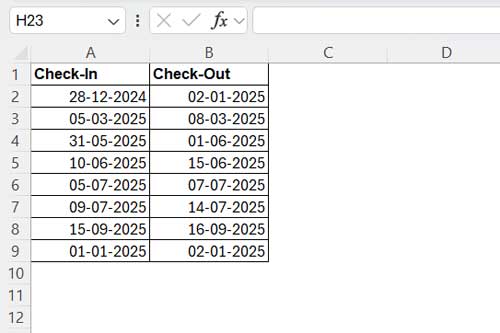
See the sample data below:

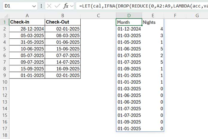
The check-in dates are in A2:A9, and the check-out dates are in B2:B9, with headers in row 1. Use the following formula in cell D1 to calculate the nights in each month:
=LET(cal,IFNA(DROP(REDUCE(0,A2:A9,LAMBDA(acc,val,LET(in,val,out,OFFSET(val,0,1),VSTACK(acc,HSTACK(EOMONTH(in,-1)+1,EOMONTH(out,-1)+1,IF(EOMONTH(in,0)<>EOMONTH(out,0),HSTACK(DAYS(EOMONTH(out,-1),in)+1,DAYS(out,EOMONTH(out,-1)+1)),DAYS(out,in))))))), 1), 0), HSTACK(VSTACK("Month", CHOOSECOLS(cal,1),CHOOSECOLS(cal,2)),VSTACK("Nights", CHOOSECOLS(cal,3),CHOOSECOLS(cal,4))))This formula will return a two-column array with the headers Month and Nights:
- The Month column contains the start dates of the months, which are date values. You should select these cells and apply date formatting by clicking Short Date within the Number group on the Home tab.
- The Nights column contains the number of nights for each month.

Note: There may be multiple occurrences of the same month depending on the bookings.
Formula Explanation
The formula calculates the number of nights for both the check-in and check-out months:
For example, if the check-in date is 28-12-2024 and the check-out date is 02-01-2025, it will return:
- 4 nights for December 2024 (from the 28th to the 31st).
- 1 night for January 2025 (on the 1st).
IF(EOMONTH(A2, 0)<>EOMONTH(B2, 0), HSTACK(DAYS(EOMONTH(B2, -1), A2)+1, DAYS(B2, EOMONTH(B2, -1)+1)), DAYS(B2, A2))The formula then appends the beginning of each month’s date:
=HSTACK(EOMONTH(A2, -1)+1, EOMONTH(B2, -1)+1, ...)This results in:
| 01-12-2024 | 01-01-2025 | 4 | 1 |
Next, we vertically stack these dates and nights into two columns:
=HSTACK(VSTACK("Month", CHOOSECOLS(...,1), CHOOSECOLS(..., 2)), VSTACK("Nights", CHOOSECOLS(..., 3), CHOOSECOLS(..., 4)))This results in:
| Month | Nights |
| 01-12-2024 | 4 |
| 01-01-2025 | 1 |
The formula uses REDUCE to apply these calculations to each date pair, returning results in a vertically stacked format. It dynamically appends the start dates of each month to ensure each calculation is correctly linked to the corresponding month.
Summarizing these results will help us effectively Calculate Nights in Each Month in Excel.
Step 2: Summarize Nights in Each Month with SUMIF or a Pivot Table
Once the nights per month are calculated, you can summarize them using either a Pivot Table or a SUMIF formula.
Calculate Nights in Each Month Using a Pivot Table
Follow these steps to create a summary:
- Select the range
D1:E17(result of Step 1). - Go to the Insert tab and click Pivot Table under the Tables group.
- Click OK to create a new worksheet with a Pivot Table layout.
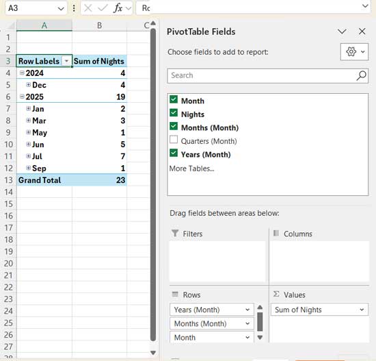
- In the Pivot Table, check Month and Nights.
- If “Quarters” appear, uncheck them to focus on months only.
You’ll get a two-column summary showing the month and the corresponding number of nights.

This is the simplest way to Calculate Nights in Each Month in Excel using a Pivot Table.
Calculate Nights in Each Month with SUMIF
If you prefer not to use a Pivot Table, you can use the SUMIF formula:
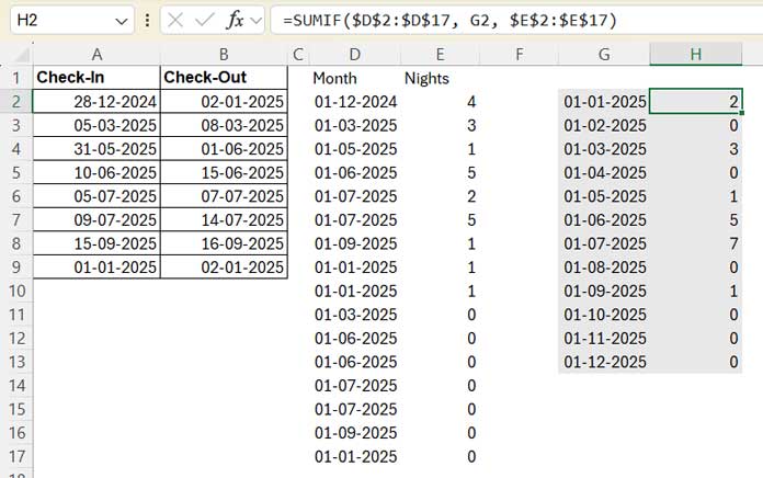
- In
G2:G13, enter the month start dates for the year you want (e.g., 01/01/2025 to 01/12/2025). - In
H2, enter the following SUMIF formula and drag it down:
=SUMIF($D$2:$D$17, G2, $E$2:$E$17)
Alternatively, for a self-expanding formula, use:
=MAP(G2:G13, LAMBDA(val, SUMIF($D$2:$D$17, val, $E$2:$E$17)))The SUMIF approach allows you to customize the month start dates and add extra columns for comments or other data.


