


I didn’t write any function related tutorials after introducing the FLATTEN. So, I think it’s high time to write one. In this tutorial let’s learn the use of the AVEDEV function in Google Sheets.
AVEDEV is a statistical function in Google Sheets. We can use this function to get the average of the magnitude of (absolute) deviations of a set of data from the mean of that set of data.
We can simply use this function with a given set of values. But that’s not enough to understand the mean deviation.
So, first, let’s see how to calculate the average deviation aka mean deviation without using the AVEDEV function in Google Sheets.
Calculating Mean Deviation in Google Sheets
In three simple steps, we can find the mean deviation of a set of values in Google Sheets. Here are those three steps.
Step # 1:
Let’s find the average deviation of the values 2, 6, 12, 14, 11, 8, 7, and 4.
The first step is to find the average of these 8 values. For that first sum the values (will get 64) and divide that sum by 8 (count of values).
So the average will be 8.
=(2+6+12+14+11+8+7+4)/8Step # 2:
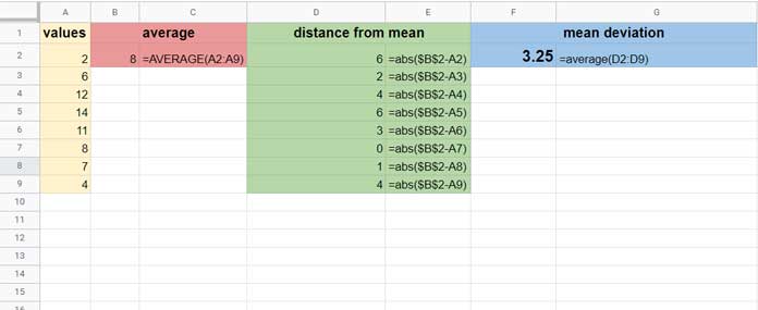
Now let’s find the absolute deviation of the values (the absolute distance/magnitude of each value) from this mean. It’s like 8-2, 8-6, 8-12…
| Values | Distance of each values from the mean (8) |
| 2 | 6 |
| 6 | 2 |
| 12 | 4 |
| 14 | 6 |
| 11 | 3 |
| 8 | 0 |
| 7 | 1 |
| 4 | 4 |
Step # 3:
Find the average of the values in column 2 which will be 3.25.
=(6+2+4+6+3+0+1+4)/8This way we can get the average deviation without using the AVEDEV function in Google Sheets.
If you use Google Sheets for the above manual calculation, it would be as below.
AVEDEV Function in Google Sheets – Syntax, Arguments, and Examples
The AVEDEV spreadsheet function in Google Sheets makes the above mean deviation calculation hassle-free.
The function calculates the average, absolute distance from the average, and finally the average of the absolute distances/deviations, all in one go.
Syntax and Arguments
Syntax:
AVEDEV(value1, [value2, ...])Arguments:
value1 – value1 is required.
value2 – optional.
You can use the values as comma-separated as per the syntax or as a reference to an array.
You can understand the same in the example section below.
Examples to AVEDEV Function in Google Sheets
Values Hard-Coded
In the first example, let’s use the above values in column A as comma-separated.
=avedev(2,6,12,14,11,8,7,4)Here if you include the Boolean TRUE/FALSE values in the AVEDEV formula, it would be counted. Like in other spreadsheet functions, the value FALSE will be treated as 0 whereas the TRUE will be treated as 1.
=AVEDEV(2,6,false,14,11,8,7,4)Any text value, text within double quotes, cause the formula to return a #VALUE error as the text can’t be coerced to a number.
If you use a named rage with the numbers, the named range should be within curly brackets.
=AVEDEV(2,6,{app},14,11,8,7,4)Values as an Array or Arrays
If you use an array, then the formula would be as below.
=avedev(A2:A9)You can use multiple arrays to include scattered values in the average deviation calculation using the AVEDEV function in Google Sheets.
Here is that example.
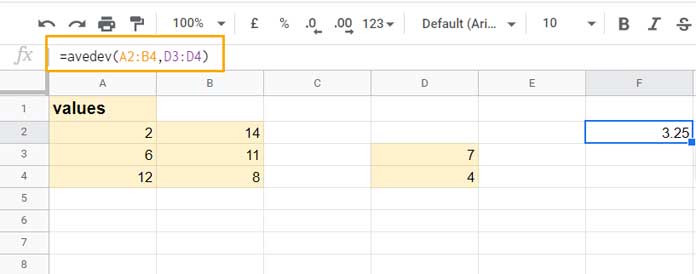
In the array use, the text values and blank cells will be ignored. So the formula won’t return any error.
That’s all about the AVEDEV function in Google Sheets.
Thanks for the stay. Enjoy!