


")


")

")
")
 in Excel & Google Sheets")


Do you want to quickly identify your least and best-selling products across all regions? It’s easy to do in Google Sheets. You can find the min or max in a Google Sheets matrix and return row data related to those values — including the product name and city — all at once.
Let’s walk through a practical example to see how this works.
Sample Data – Car Sales by City
Assume you have the following car sales data:
| Type | Bangalore | Mumbai | Cochin | Hyderabad |
| Sedan | 450 | 700 | 465 | 375 |
| SUV (Sport Utility Vehicle) | 300 | 450 | 222 | 300 |
| Hatchback | 420 | 800 | 10 | 100 |
| Coupe | 75 | 200 | 5 | 80 |
| Convertible | 12 | 27 | 4 | 13 |
| Wagon (Estate Car/Station Wagon) | 2 | 8 | 2 | 4 |
| Minivan (MPV – Multi-Purpose Vehicle) | 4 | 12 | 1 | 10 |
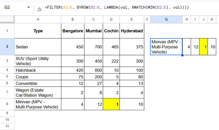
Let’s say you want to find the minimum car sales across the entire matrix and return the entire row of that product. This way, you not only get the sales figure but also the car type and the city it belongs to — all in one go.
Example – Find the Minimum Sales and Return Row Data
From the above data, the formula would return:
Minivan (MPV - Multi-Purpose Vehicle) | 4 | 12 | 1 | 10
Here, the lowest value is 1, which appears under Cochin, making it clear that Minivan had the least number of sales in that city.
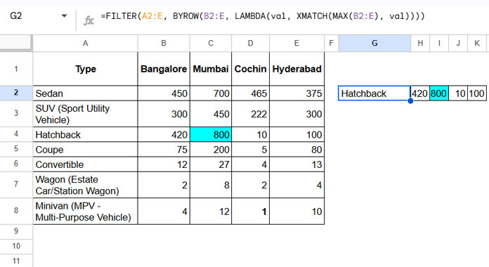
Example – Find the Maximum Sales and Return Row Data
If you’re looking for the highest sales:
Hatchback | 420 | 800 | 10 | 100
The maximum value is 800, which is under Mumbai, and the product is Hatchback — the best-selling model.
Formula to Find the Minimum Value and Return Row Data in Google Sheets
=FILTER(A2:E, BYROW(B2:E, LAMBDA(val, XMATCH(MIN(B2:E), val))))This formula allows you to find the min in a matrix and return the corresponding row (or rows, if there are multiple matches) in Google Sheets.
How the Formula Works
MIN(B2:E)finds the lowest value in the matrix.BYROW(..., LAMBDA(...))checks each row to see if it contains that min value.XMATCH(..., val)returns TRUE if the min is found in that row.FILTER(...)then pulls the matching row(s) fromA2:E.
Formula to Find the Maximum Value and Return Row Data in Google Sheets
=FILTER(A2:E, BYROW(B2:E, LAMBDA(val, XMATCH(MAX(B2:E), val))))This version works the same way as the min formula, but uses MAX instead to return the row with the highest value in the matrix.
Optional – Append Headers to the Output
To enhance readability, you can also include headers above the returned row using VSTACK:
=VSTACK(A1:E1, FILTER(A2:E, BYROW(B2:E, LAMBDA(val, XMATCH(MIN(B2:E), val)))))Or for max:
=VSTACK(A1:E1, FILTER(A2:E, BYROW(B2:E, LAMBDA(val, XMATCH(MAX(B2:E), val)))))This displays both the headers and the result in one neat table.
Conclusion
Finding the min or max in a Google Sheets matrix and returning row data can be incredibly useful for analysis. Whether you’re tracking sales, performance, or scores, this method helps you pull contextual data from complex tables with just one formula.
Related Tutorials
If you’re interested in more matrix-based lookups and manipulations, check out these posts: