Google Sheets: Highlight Multiple Tables on the Same Sheet

If you’ve used tables in Google Sheets (via Insert > Pre-built tables or right-click > Convert to table), you may have noticed that highlighting one table doesn’t work the way you’d expect when there are multiple tables on the same sheet.

Why? Because conditional formatting in Google Sheets doesn’t support structured table references. You can’t apply a rule using the table name, and if you select a full column range (like A1:C), the formatting might spill over into other tables in that area.

So when you try to highlight multiple tables on the same sheet in Google Sheets, things get messy. Luckily, there’s a clean workaround.

Table of Contents

Quick Solution to Highlight Multiple Tables in Google Sheets

To highlight multiple tables on the same sheet without overlap, use helper columns with array formulas and apply conditional formatting based on those helper values.

Real-Life Scenario: Team Reports in a Single Sheet

Imagine you’re managing a small business with three teams: Sales, Support, and Marketing.

You collect each team’s monthly data in separate blocks on the same sheet:

Sales Table (A1:C4)

Name	Target	Achieved
Alice	100	110
Diya	90	85

Support Table (A8:C11)

Name	Tickets Handled	Resolution %
Zara	50	92%
Dave	45	95%

Marketing Table (A15:C18)

Name	Campaigns	Leads
Saanvi	5	300
Frank	4	250

Each table starts at a different spot (A1, A8, A15). You want to:

Apply unique highlight rules to each table
Ensure the formatting adjusts when rows are added
Avoid rules from spilling into other tables

Why Conditional Formatting Overlaps Across Multiple Tables

If you apply a conditional format to a fixed range like A1:C4, it won’t include new rows when the table grows.
If you apply the rule to A1:C, it will extend down through all rows in those columns — potentially overlapping with other tables on the same sheet.

So what’s the solution?

How to Highlight Multiple Tables in Google Sheets

We’ll use helper columns next to each table to control the formatting — no overlap, no hassle.

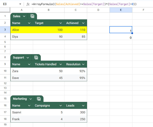
1. Highlight Achievers (Sales Table)

Let’s highlight names where the Achieved value is greater than or equal to Target.

We’ll use column E as a helper column for the Sales table.

In cell E3, enter:

=ArrayFormula((Sales[Achieved]>=Sales[Target])*(Sales[Target]>0))

This returns 1 for rows where targets are met. The best part? As the table grows, the formula expands automatically.

Highlighted rows in the Sales table where the Achieved value meets or exceeds the Target in Google Sheets

Now apply the conditional format:

Select range A3:C
Go to Format > Conditional formatting
Under “Custom formula is”, enter
=$E3=1
Choose a highlight color
Click Done

Only rows in the Sales table will be highlighted — no overlap.

2. Highlight High Resolution Rates (Support Table)

Now let’s highlight rows in the Support table where resolution percentage is above 90%.

Use column F as the helper column.

In cell F10, enter:

=ArrayFormula(Support[Resolution %]>90%)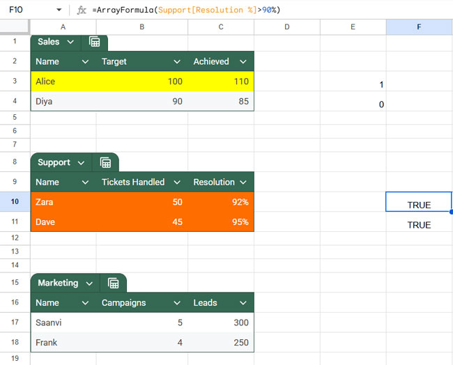

Conditional formatting applied to the Support table in Google Sheets to highlight resolution rates above 90%

Then:

Select range A10:C
Go to Format > Conditional formatting
Click “Add another rule”
Set rule type to Custom formula is
Enter: =$F10=TRUE
Pick a different highlight color
Click Done

Now only the Support table is affected.

3. Apply the Same Method to Other Tables

You can repeat the same technique for the Marketing table or any additional blocks. Just use a different helper column and adjust the row references.

This method works perfectly to highlight multiple tables on the same sheet in Google Sheets, even as data grows or changes.

Why This Method Works for Multiple Tables in Google Sheets

Helper columns isolate logic to each table
Array formulas grow with the table
Custom formulas let you apply precise rules to the right rows
No overlapping or conflicting highlights

Common Mistakes When Highlighting Multiple Tables

❌ Applying rules to entire columns (e.g., A:C)
This causes formatting to spill into other tables on the same sheet.
❌ Not using helper columns
Without helper columns, it’s difficult to isolate conditions for each table, leading to overlapping or incorrect highlights.
❌ Using fixed ranges that don’t expand
Applying rules to a fixed range like A1:C4 won’t include new rows when the table grows.
❌ Incorrect row references in custom formulas
Using the wrong starting row (e.g., $E1 instead of $E3) can misalign the formatting.
❌ Mixing multiple table rules in one condition
Trying to handle multiple tables in a single formula often leads to complex and unreliable rules.

Conclusion

Highlighting multiple tables on the same sheet in Google Sheets can be tricky because conditional formatting doesn’t support structured table references directly. However, by using helper columns and array formulas, you can apply precise, non-overlapping rules that scale as your data grows.

This approach is especially useful when managing multiple data blocks like team reports, dashboards, or segmented datasets within a single sheet.

This tutorial is part of The Ultimate Guide to Conditional Formatting in Google Sheets, where you can explore more formatting techniques, practical examples, and advanced use cases to better organize and analyze your data.