In this post, you’ll learn how to generate barcodes in Google Sheets, both single and multiple, using the Code 39 standard.

What Is Code 39?

Code 39 is a barcode symbology that allows encoding of:

• Numbers (0-9)
• Uppercase letters (A-Z)
• Special characters: space, dollar sign ($), percent (%), forward slash (/), period (.), plus (+), and minus (-)

Note: The asterisk * is also part of the Code 39 character set, but it serves a special role — it acts as the start/stop delimiter in each barcode.

You might want to generate or create barcodes in Google Sheets for various reasons. Barcodes are machine-readable, help reduce human error, and save time — especially when managing inventory or labeling items.

Let’s skip the benefits and jump into how to create barcodes in Google Sheets.

Steps to Generate Barcodes in Google Sheets

Let’s walk through how to generate Code 39 barcodes in Google Sheets using a real-world example — say, a list of landscaping materials.

Step 1: Basic Settings (Sheet1)

1. In column A (A2:A), enter your item descriptions.
2. In column B (B2:B), enter item codes using:
   • Letters A-Z
   • Numbers 0-9
   • The seven special characters mentioned earlier (excluding the asterisk *)
     Tip: While Code 39 doesn’t have a strict character limit, it’s best to keep item codes under 25 characters. Longer codes can make the barcode too wide and may not scan reliably, especially on smaller labels or printers.
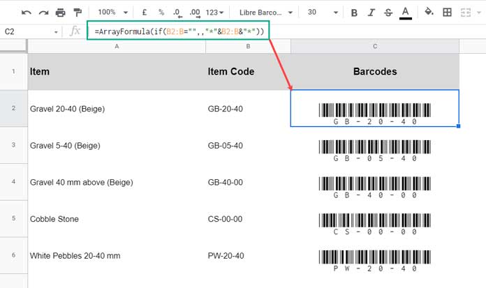
3. In cell C2, insert the following formula to create barcodes:

=ArrayFormula(IF(B2:B="",, "*" & B2:B & "*"))

Why use the asterisk *?

For example, let’s say item A2 is “Gravel 20-40 (Beige)” and its code in B2 is GB-20-40. The formula transforms it into *GB-20-40*, which includes the start/stop symbols necessary for barcode scanners to identify the beginning and end of the code.

Step 2: Formatting for Barcode Display

Formatting is critical to making your generated barcodes scannable.

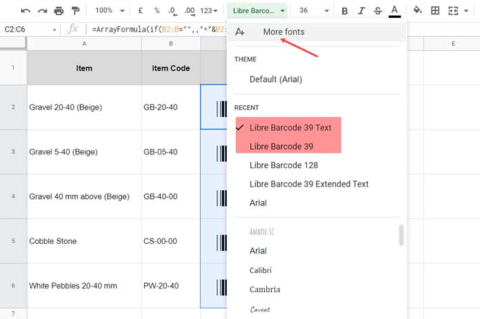
1. Select column C2:C (the barcode column).
2. Click the Font drop-down from the toolbar and select:
   • Libre Barcode 39
   • Or Libre Barcode 39 Text (If not available, click More Fonts and search for it.)
3. Set the Font Size to 39 for better visibility.

At this point, you’ve successfully created barcodes in Google Sheets using Code 39!

Note:

Google Sheets offers two fonts for Code 39: Libre Barcode 39 and Libre Barcode 39 Text.

• Libre Barcode 39 displays only the bars (no human-readable text).
• Libre Barcode 39 Text includes both the barcode and the readable text below it.

Choose the one that fits your labeling needs — for example, use Libre Barcode 39 Text if you want both machine and human readability.

How to Repeat Barcodes N Times in Google Sheets

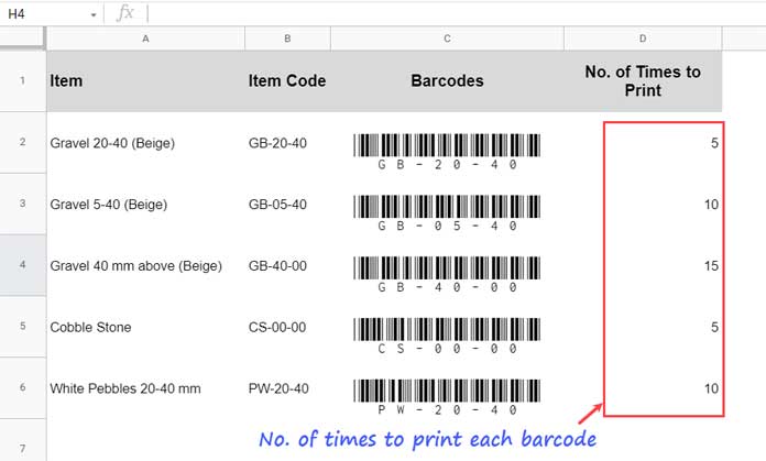
What if you want to print each barcode multiple times — say, for labeling?

For instance:

• Gravel 20-40 (Beige): 5 copies
• Gravel 5-40 (Beige): 10 copies
  …and so on.

Here’s how to repeat barcodes in Google Sheets based on quantity.

Step-by-Step Instructions:

1. In Sheet1!D2:D, enter the number of times each barcode should be repeated.
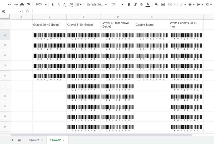
2. Add a new sheet (Sheet2) by clicking the + button.
3. In Sheet2!B1, insert this formula to list the item descriptions horizontally:

=TRANSPOSE(FILTER(Sheet1!A2:A6, Sheet1!A2:A6 <> ""))

4. In Sheet2!B2, insert the following array formula to repeat the generated barcodes:

=ArrayFormula(
     TRANSPOSE(
        SPLIT(
           REPT(
              FILTER(Sheet1!C2:C & "♡", Sheet1!C2:C <> ""),
              FILTER(Sheet1!D2:D, Sheet1!C2:C <> "")
           ),
           "♡"
        )
     )
)

This formula uses:

• REPT to repeat the barcodes
• SPLIT with a unique delimiter (♡) to separate values
• TRANSPOSE to lay out the repeated barcodes correctly

5. Format cells B2:F with the Libre Barcode 39 Text font and set the font size to 36.
6. Adjust spacing if needed and print your barcode labels.

Can You Lookup Decoded Code 39 Barcodes?

Yes, absolutely! Once you’ve generated barcodes in Google Sheets, you might want to lookup a decoded barcode to get the item description or other details.

Here’s How:

Let’s say in Sheet3!A1, you have a decoded barcode value like "GB-05-40".

Your lookup table is in Sheet1!A2:B — with descriptions in column A and item codes in column B.

To perform a lookup, insert this XLOOKUP formula in Sheet3!B1:

=XLOOKUP(A1, Sheet1!B2:B, Sheet1!A2:A, "")

This performs a lookup on column B (Item Code) and returns the corresponding description from column A.

To look up a list of barcodes (say, in column A), use an array formula in B1:

=ArrayFormula(XLOOKUP(A1:A, Sheet1!B2:B, Sheet1!A2:A, ""))

Conclusion

That’s everything you need to know to generate barcodes in Google Sheets using the Code 39 format — including repeating them, formatting correctly, and even lookups.

Whether you’re managing inventory, printing labels, or organizing assets, this method provides a simple, efficient solution — all within Google Sheets.

Thanks for reading. Happy barcode generating!