If you’re managing leaves for a team—or just trying to keep better tabs on your own time off—this free Employee Annual Leave Tracker in Google Sheets can seriously simplify things. Pick an employee from a dropdown, select the year and starting month, and the calendar automatically updates.

You’ll see all 12 months at a glance, with weekends, working days, and leave types like Casual, Sick, or Maternity Leave neatly color-coded. There’s even a tidy little summary of total leaves taken and networking days for the selected year.

Whether you’re in HR, managing a team, or just want to stop digging through messy sheets, this template gives you a clean, interactive way to visualize time off.

Preview & Download the Template

Why Use This Employee Annual Leave Tracker in Google Sheets?

Here’s why I built (and actually use) this tracker in Google Sheets:

1. Quick Employee, Year & Starting Month Selection

Just pick an employee, choose the year and starting month (calendar or financial year), and you’re done—no formulas to update, no scrolling through tabs. Everything refreshes instantly.

2. Color-Coded Leave Types

Each leave type has its own color so it’s easy to spot what kind of leave was taken. Casual Leave and Sick Leave don’t blend together anymore.

3. See the Entire Year in One Sheet (Calendar or Financial)

No flipping between months or tabs. The full 12-month period—whether January–December or April–March—is displayed on a single page.

4. Leave Summary Built Right In

See a breakdown of leave types taken and total networking (i.e., working) days for the year. It updates based on your selections.

5. Reusable Year After Year

Change the year or starting month, and the calendar rebuilds itself with correct dates and weekday alignment. One dynamic setup powers the entire sheet—no clutter.

6. 100% Google Sheets

No apps, no integrations, no fuss. It’s all in Google Sheets and fully editable if you want to make tweaks.

7. Easy to Customize

If you’re feeling adventurous, you can customize the leave types and even change which days count as weekends. I cover how that works in the next section.

Note: The screenshot above is from version 0. The new version (v2) includes updates such as the month selector and improved financial year support.

How to Use the Employee Annual Leave Tracker Template

Here’s how to get started with the tracker.

1. Update Your Employee List

Head to the ‘List of Employees’ tab.

• Delete the dummy names in column A (starting from A2)
• Add your own employee names

2. Enter Your Holiday List

Go to the ‘Holiday List’ tab.

• Remove the sample dates in column A
• Add your actual holidays in column A, and optionally describe them in column B
• These holidays will be excluded from working day counts

You can include multiple years of holidays or just the current year—it’s up to you.

3. Leave Types

The ‘Leave Types’ tab is pre-filled. You don’t need to change anything for it to work. If you want to customize leave types later, I explain how in the formula section.

4. Enter Leave Data

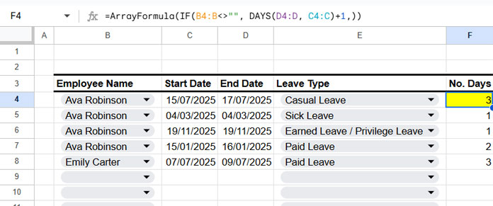
This part lives in the ‘Leave Data’ tab.

• Clear the sample data in B4:E
• In B4, pick an employee
• In C4 and D4, enter the start and end dates
• In E4, choose the leave type
• Columns F and G automatically calculate the number of leave days — Column F shows the total days taken, while Column G shows the number of days within the current year.

Add more rows as needed.

5. Check the Calendar

Now head to the ‘Calendar’ tab.

• In C2, choose the employee you want to check
• In C3, select the year
• In I3, choose the starting month (January for a calendar year, or another month for a financial/fiscal year)

That’s it—the calendar updates with all their leave info:

• Rows 2 and 3 (starting from column M) show the leave type summary
• Range C6:AM17 contains the monthly calendar view
• Leave days are highlighted in different colors
• Networking (working) days are shown in light grey
• Weekends are excluded by default (Saturday and Sunday)
• The total number of networking days is shown in D19

How It Works (Formulas and Rules Explained)

Month Start Dates (Cell B6 in ‘Calendar’)

The following formula generates month start dates for the selected month and year in the range B6:B17. The result is then formatted as MMM-YY.

=ArrayFormula(EDATE(EDATE(DATE(C3, I3, 1), -1), SEQUENCE(12)))

This ensures the calendar aligns correctly with the chosen start month, supporting both financial and regular calendar years.

Calendar Formula (Cell C6 in ‘Calendar’)

Here’s the formula that builds the full calendar with proper date alignment for the selected start month and year:

=IFNA(
   MAP(
      B6:B17, 
      LAMBDA(r, 
         LET(
            seq, SEQUENCE(1, DAY(EOMONTH(r, 0)), r), 
            offset, TOROW(WRAPCOLS(,WEEKDAY(r)), 1), 
            HSTACK(offset, seq)
         )
      )
   )
)

This formula builds the calendar based on the month start dates in B6:B17, generating the correct number of days and weekday alignment for each month. If the calendar doesn’t display correctly, check the values in B6:B17 first.

Working Day Highlights (Light Grey)

This rule shades working days (excluding weekends and listed holidays):

=AND(NOT(OR(WEEKDAY(C6)=1, WEEKDAY(C6)=7)), ISNA(XMATCH(C6, INDIRECT("Holiday List!A2:A"))))

Note: You can view or edit this rule by clicking anywhere in the calendar grid, then going to Format → Conditional formatting from the menu.

Here, WEEKDAY(C6)=1 represents Sunday, and WEEKDAY(C6)=7 represents Saturday — meaning Saturday and Sunday are treated as weekends.

👉 To modify:
Change the numbers inside the OR() to match your weekend days based on the WEEKDAY numbering system
(default is 1 = Sunday, 2 = Monday, … 7 = Saturday).

Examples:

• For Friday–Saturday weekends: OR(WEEKDAY(C6)=6, WEEKDAY(C6)=7)
• For Sunday only: OR(WEEKDAY(C6)=1)
• For Friday only: OR(WEEKDAY(C6)=6)
• For Sunday–Monday weekends: OR(WEEKDAY(C6)=1, WEEKDAY(C6)=2)

Adjust the numbers as needed to match your organization’s weekend setup.

Leave Type Highlights

There are 8 leave types by default:

• Casual Leave
• Compensatory Off (Comp-Off)
• Earned Leave / Privilege Leave
• Maternity Leave
• Paid Leave
• Paternity Leave
• Sick Leave
• Unpaid Leave

Each one has its own highlight rule. Here’s the one for Sick Leave:

=LET(
   ftr, FILTER(
      INDIRECT("Leave Data!C4:D"), 
      INDIRECT("Leave Data!B4:B")=$C$2, 
      INDIRECT("Leave Data!E4:E")="Sick Leave"
   ), 
   COUNTIF(
      MAP(CHOOSECOLS(ftr, 1), CHOOSECOLS(ftr, 2), LAMBDA(start, end, ISBETWEEN(C6, start, end))), 
      TRUE
   )
)

Note: This is a conditional formatting rule. To view or edit it, click any cell in the calendar grid, then go to Format → Conditional formatting. You’ll see separate rules for each leave type (Sick Leave, Paid Leave, etc.).

I’ve duplicated this rule 8 times—once for each leave type—and just updated the text "Sick Leave" (or "Paid Leave", etc.) inside the formula.

So, if you modify the leave types listed in the ‘Leave Types’ sheet, make sure to update these 8 highlight rules as well. You only need to change the leave type name in each formula—nothing else.

Leave Summary (Rows 2 and 3)

Example formula in P2 for Casual Leave:

=SUMIFS('Leave Data'!$G$4:$G, 'Leave Data'!$E$4:$E, M2, 'Leave Data'!$B$4:$B, $C$2)

This formula uses the label in M2 (which is “Casual Leave” by default) to calculate the leave total. The structure is the same across Row 2 and Row 3.

So, if you customize the leave types in the ‘Leave Types’ sheet, make sure to update the labels in Rows 2 and 3 accordingly. You don’t need to touch the formulas—just ensure the labels match your updated leave types exactly.

Networking Day Count (D19)

This shows the total working days in the selected year:

=NETWORKDAYS.INTL(B6, EOMONTH(B17, 0), "0000011", 'Holiday List'!A2:A)

Here, “0000011” defines the weekend pattern — each digit represents a day from Monday (first) to Sunday (last), where:

• 0 = working day
• 1 = weekend

So "0000011" means Saturday and Sunday are weekends.

👉 To modify:

• For Friday–Saturday weekends, use "0000110"
• For Sunday only, use "0000001"
• For Friday only, use "0000100"
• For Sunday–Monday weekends, use "1000001"

Adjust the pattern according to your organization’s weekend schedule.

Calculating Leave Days Automatically

Column G in ‘Leave Data’ uses:

=VSTACK(
  "No. Days in the Current Year",
  ARRAYFORMULA(
    LET(
      d,
      DAYS(
        IF(D4:D <= EOMONTH(Calendar!B17, 0), D4:D, EOMONTH(Calendar!B17, 0)),
        IF(C4:C >= Calendar!B6, C4:C, Calendar!B6)
      ) + 1,
      IF(d > 0, d, )
    )
  )
)

This counts the total number of days taken per entry in the selected year.

FAQs

Can I add custom leave types?
Yes, but you’ll need to update the conditional formatting rules and summary row headers to match the new names.

How do I change weekends?
There are two places where weekends are handled, and they work differently:

1. Calendar highlights (networking days) – This uses WEEKDAY(C6) in the conditional formatting rule. By default, it excludes Saturdays (7) and Sundays (1). If your weekends are different (like Friday and Saturday), update the WEEKDAY(C6) part in the formula accordingly.
2. Total working days (cell D19) – This uses the NETWORKDAYS.INTL function, which relies on a 7-digit pattern where each digit represents a weekday (Monday to Sunday). A 1 marks a weekend, and a 0 marks a working day.
   • For example, "0000011" means Saturday and Sunday are weekends.

So if you’re changing weekends, you’ll need to adjust both: the WEEKDAY() logic in the calendar highlight rule and the weekend pattern string in the NETWORKDAYS.INTL formula.

Can I see multiple employees together?
This template shows one employee at a time. You could duplicate the calendar sheet for each employee or build a dashboard if needed.

Want to see it in action? Watch the video below. You can download the template from the link above.

Conclusion

This Employee Annual Leave Tracker in Google Sheets makes it easy to track leave with a clean, automated setup. Everything updates based on your input—no coding needed. Whether you’re managing a team or your own time off, it helps you stay organized without the usual spreadsheet mess.

Changelog

Track updates and improvements to the template over time.

v2.0 — Dec 2025
Added support for financial/fiscal years by allowing users to select both the year and the starting month. Updated calendar formulas and calculations accordingly.

v1.1 — Nov 2025
Added a new VSTACK + ArrayFormula in the “No. Days [Year]” column of the Leave Data sheet to calculate leave days within the selected year.

v1.0 — Initial Release
Employee Annual Leave Tracker template launched.

Resources

• Advanced Employee Annual Leave Tracker Template in Excel (Free Download)
• Free Automated Employee Timesheet Template for Google Sheets
• Google Sheets Payroll Template: Service Days Calculator with Custom Leave
• Create a Habit Tracker in Google Sheets: Step-by-Step Guide
• Array Formula to Split Group Expenses in Google Sheets