Google Sheets doesn’t provide a direct way to delete hidden rows. That’s usually fine—until you start filtering data or hiding rows and later need to clean things up.
At that point, simply “select and delete” doesn’t work the way you expect.
Over time, I found a more reliable approach: use a helper column to identify hidden rows first, then delete them safely.
This method works whether your rows are:
- hidden by filters
- manually hidden
- or a mix of both
Why Not Just Unhide and Delete?
That’s the obvious approach—but it breaks down quickly.
- If you’re using filters, unhiding isn’t even relevant
- If you have a large dataset, manually checking rows is slow
- You risk deleting the wrong rows if visibility changes
So instead of guessing, it’s better to mark the rows first.
The Idea Behind This Method
The goal is simple:
Don’t delete blindly. First identify which rows are hidden.
To do that, we use:
- a sequence column (to give each row a reference)
- the SUBTOTAL function (to detect visibility)
Once each row is marked as visible or hidden, deletion becomes straightforward.
Example: Cleaning a Simple Dataset
Here’s a small example:
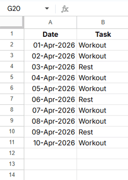
Let’s say you filter out rows where Task = “Rest” and later decide to remove those rows completely.
Method 1: Delete Rows Hidden by Filter
Step 1: Apply Your Filter
Filter column Task and exclude “Rest”.
Now those rows are hidden—but not deleted.
Step 2: Add a Sequence Column
In an empty column (say column D), enter the following formula in cell D1:
=SEQUENCE(ROWS(A1:A))This simply assigns a number to each row.
We use the helper column (D) so that each row has a numeric reference for SUBTOTAL to evaluate reliably.
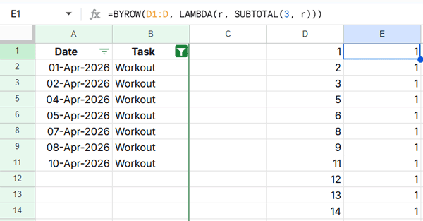
Step 3: Mark Visible vs Hidden Rows
In cell E1, enter:
=BYROW(D1:D, LAMBDA(r, SUBTOTAL(3, r)))Now each row will return:
- 1 → visible
- 0 → hidden (filtered out)
At this point, you’ve effectively “revealed” which rows were hidden.
Step 4: Lock the Results
Copy column E and paste it back as values only (Right-click → Paste special → Values only).
Why this matters:
If you skip this step, the results will change when you remove the filter—making it impossible to target the correct rows.
Step 5: Delete the Hidden Rows
- Remove the filter
- Apply a new filter on column E
- Uncheck 1 to make only the rows to delete visible
- Select those rows → Right-click → Delete selected rows
- Remove the filter
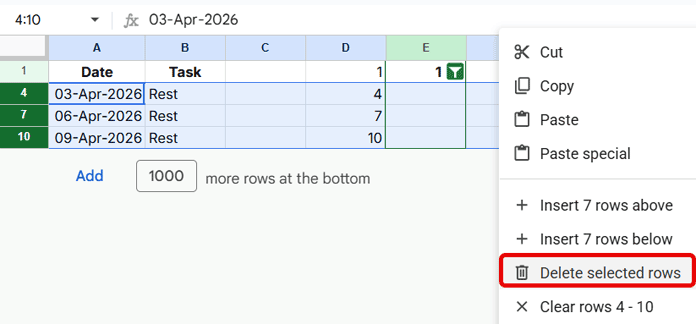
Done. The previously hidden rows are now gone.
Method 2: Delete Filtered + Manually Hidden Rows
Things get slightly more interesting when your sheet includes manually hidden rows as well.
The previous formula won’t catch those.
Use This Formula Instead
=BYROW(D1:D, LAMBDA(r, SUBTOTAL(103, r)))The difference is subtle but important:
3→ counts only visible rows (ignores filtered-out rows)103→ counts only visible rows (ignores both filtered and manually hidden rows)
Important Step: Unhide Before Deleting
When rows are manually hidden, they can’t be selected—even if your helper column identifies them.
After converting results to values:
- Select all rows
- Right-click → Unhide rows
- Remove the filter
This doesn’t undo your work—it simply ensures those rows are selectable for deletion.
Then:
- Apply a filter on column E
- Uncheck 1
- Select the visible rows → Delete selected rows
Method 3: Only Manually Hidden Rows
If you’re dealing only with manually hidden rows:
- First remove any filters
- Then use the same
103formula
Everything else stays the same.
A Small but Important Mistake to Avoid
One thing that can go wrong here:
Forgetting to convert formulas to values.
For Methods 1 and 2, if you remove the filter before doing that:
- The formula recalculates
- Hidden rows may appear as visible
- You end up deleting the wrong rows
For Method 3 (manually hidden rows only), removing the filter first is required—but you should still convert the results to values before proceeding with deletion.
This is the one step you shouldn’t skip.
Why This Approach Is Reliable
What makes this method work is the behavior of SUBTOTAL:
- It reacts to row visibility
- It treats filtered and manually hidden rows differently (based on the function code)
- It can be applied row-by-row using BYROW
Instead of relying on what you see, you’re working with a clear marker.
When I Use This Method
I typically use this when:
- Cleaning filtered datasets
- Removing excluded categories (like “Rest” in this example)
- Preparing data for analysis where row count matters
Once you get used to it, it’s faster than manual cleanup.
Final Thoughts
There’s no one-click option to delete hidden rows in Google Sheets—but you don’t really need one.
By marking rows first and then deleting them, you:
- avoid mistakes
- keep control over your data
- and get consistent results every time
It’s a simple shift in approach—but it saves a lot of headaches once your datasets grow.


