Arrange Numbers into Low, Medium, and High in Google Sheets

When working with datasets, you may want to arrange numbers into Low, Medium, and High categories to quickly spot trends or group values for analysis. Google Sheets doesn’t have a direct function for this, but with a clever formula, we can classify any array of numbers into these three groups.

In this tutorial, you’ll learn step-by-step how to use the PERCENTRANK function with FILTER to split your data into Low, Medium, and High ranges. You’ll also learn how to check if a specific number belongs to one of these categories without manually scanning your dataset.

Table of Contents

Why Arrange Numbers into Low, Medium, and High in Google Sheets?

Categorizing numbers helps in:

Understanding distribution of data at a glance.
Simplifying reports by grouping values.
Highlighting performance levels or priority ranges.

Instead of manually separating values, you can use a formula-based approach so the grouping updates automatically whenever the dataset changes.

Arrange Numbers into Low, Medium, and High in Google Sheets (Step-by-Step)

Suppose you have the following numbers in A2:A:

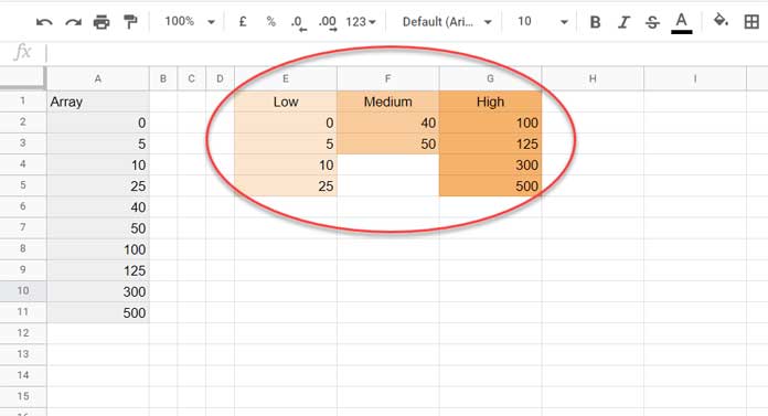
Sample data with expected Low, Medium, and High categories in Google Sheets

We’ll use three formulas — one each for Low, Medium, and High — placed in E2, F2, and G2 respectively.

1. Calculate Percentile Rank for Each Number

First, insert the following formula in C2:

=ArrayFormula(PERCENTRANK(A2:A, A2:A))

Google Sheets column showing percentile ranks calculated with PERCENTRANK formula

This returns the percentile rank of each value in the dataset.

The minimum value gets a percentile of 0.
The maximum value gets a percentile of 1.
Other values fall between 0 and 1.

2. Filter Numbers into Low, Medium, and High Groups

We’ll use the following logic:

Low → Percentile rank ≤ 1/3
Medium → Percentile rank > 1/3 and ≤ 2/3
High → Percentile rank > 2/3

Low (E2)

=FILTER(A2:A, C2:C <= 1/3)

Medium (F2)

=FILTER(A2:A, C2:C > 1/3, C2:C <= 2/3)

High (G2)

=FILTER(A2:A, C2:C > 2/3)

You can also replace C2:C in each formula with the PERCENTRANK formula directly and remove the helper column entirely.

Test Whether a Value Falls in Low, Medium, or High in a Range

Sometimes you only need to test one number to see which category it belongs to. For this, we can use IF with PERCENTRANK.

IF formula in Google Sheets testing percentile rank to return Low, Medium, or High

Formula to Find the Position of a Number in an Array

Suppose the number to test is in H2. Use this in I2:

=IFNA(
  IF(PERCENTRANK(A2:A, H2) <= 1/3, "Low",
     IF(PERCENTRANK(A2:A, H2) <= 2/3, "Medium", "High")
  ),
  "Number Doesn't Exist in the Array"
)

Logic:

Percentile ≤ 0.333 → Low
Percentile > 0.333 and ≤ 0.666 → Medium
Percentile > 0.666 and ≤ 1 → High
Above 1 → Number not found in the dataset

Conclusion

With PERCENTRANK and FILTER, you can easily arrange numbers into Low, Medium, and High in Google Sheets without manual sorting. This approach is dynamic — if your dataset changes, the categories update automatically.