You may want to format numbers using your country’s currency format in Google Sheets, especially when you are working locally.
Currency formatting is a type of accounting number format that prefixes a chosen currency to a number. I use currency formatting when I make cash flows and regular number formatting when I prepare measurements of my work.
The default currency format in your spreadsheet may be US dollars or some other currency, depending on your spreadsheet settings. Let’s see how to use your country’s currency format in Google Sheets.
The easiest way to set your country’s currency format as the default currency in Google Sheets is as follows:
- Click Sheets.new to open a blank spreadsheet.
- Click File > Rename and name it something like “Default Sheet” or any other name that you can remember easily.
- Click File > Settings.
- Under Locale, select your country.
- Optionally, under Time Zone, choose your time zone.
- Click Save and Reload.
- Close the window.
Whenever you want to create a new sheet, open this file and, from the File menu, make a copy of it. This way, you can easily apply your country’s currency format in Google Sheets. Here’s how:
How to Format Numbers in Google Sheets with Your Country’s Currency Symbol
In the previous step, we set the currency format to our country’s currency format. Let’s say I chose “India” as the country under locale. How do I format numbers in A2:A10 with “Rs” as the currency symbol, which is my default currently?
To do this, select the cell range A2:A10, which contains the numbers you want to format. Then, click Format > Number > Accounting/Currency/Currency rounded. This will apply your country’s currency formatting in Google Sheets.
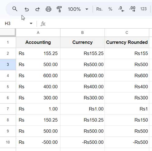
Accounting, Currency, and Currency rounded will all add your country’s currency symbol to the number. However, they differ slightly:
- In accounting format, the currency symbol is left-aligned and the numbers are right-aligned within the cell.
- In currency and currency rounded, the symbol is prefixed to the number and there is no packing. Instead, it is aligned to the right altogether.
Please see the following illustration to understand the difference:
Note: As the name suggests, currency formatting only changes the visual appearance of the numbers formatted. The underlying values will remain the same. Therefore, the rounding in “Currency rounded” is only visual. If you want to round your numbers, use the ROUND function.
How to Use Foreign Currency Formats in Google Sheets
If you don’t want to format numbers in Google Sheets with your own country’s currency format, you can follow these steps:
- Assume you want to use Japanese Yen (¥) as the currency format and your default currency is different.
- Select the cell or range of cells that you want to format with a foreign currency (here, Japanese Yen).
- Click Format > Number > Custom currency.
- Enter the first few letters of the currency, for example, “jap”, in the field.
- Google Sheets will show the available formatting. Select the one you want and click Apply.
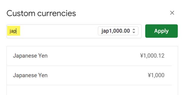
As you can see, this shows only the Currency and Currency rounded formatting of a foreign currency.
How to Format Foreign Currency in Google Sheets with Accounting Style
My country’s currency format is set to Rs. in Google Sheets. Here is how to use a different currency format in an accounting style, using Japanese Yen as an example:
Assume the number to format is in cell range A2:A10.
Select cell range A2:A10.
Apply the “Currency” formatting following the above steps (Go to Format > Number > Custom Currency > Select Japanese Yen).
Click Apply.
In cell D1 or any blank cell, enter =LEFT(A2,1) to extract the currency symbol from the amount.
Copy the symbol from cell D1 and in the following code replace the text your_symbol with the copied currency symbol:
_-[$your_symbol-420]* #,##0.00_-;_-[$your_symbol-420]* \-#,##0.00_-;_-[$your_symbol-420]* "-"??_-;_-@Since I want Japanese Yen, my code after replacing the text your_symbol with ¥ will be as follows:
_-[$¥-420]* #,##0.00_-;_-[$¥-420]* \-#,##0.00_-;_-[$¥-420]* "-"??_-;_-@Copy this code.
Select cell range A2:A10.
Click Format > Number > Custom number format.
Replace the existing code with the just copied code and click Apply.
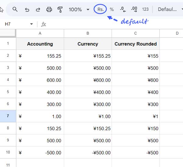
This way, you can get accounting format with a foreign currency in Google Sheets.
Conclusion
What should I do if my currency symbol is not available in Google Sheets?
There is another workaround to get any currency format into your Google Sheets. You can format your number with custom text. This means that you can suffix or prefix currency text to the number, which will also keep or retain the number format.
Here are some tips on how to add custom text to a number that can be considered in calculation: How to Add Custom Text to Number that Can be Considered in Calculation.
To convert currency, you can use the GOOGLEFINANCE function in Google Sheets.


Hi
This only selects the RS but format is still US style 1,000,000 not Indian 1,00,000. Any idea how to change that.
Thanks
You can use the custom number format in this case.
Format>Numbers>More Formats>Custom Number Format
Sorry for the late reply