We can automate age analysis using pivot tables in Google Sheets with the only prerequisite being well-formatted data.
Age analysis is a data analytic method used to categorize and evaluate data based on age-related parameters.
In this tutorial, we will analyze the aging of invoices or payments due from customers. This helps in managing and tracking overdue payments effectively.
This tutorial is part of our complete Google Sheets Pivot Table Tutorial, which covers pivot table basics, setup, and advanced date grouping techniques.
Prepare Your Data for Age Analysis
Creating a pivot table doesn’t require any expertise. The key is having a well-formatted accounts receivable statement to start from.
You can refer to the following format for the accounts receivable statement:
Customer Name | Invoice # | Invoice Date | Due Date | Amount DueArrange the data accordingly in cell range A1:E in a blank sheet.
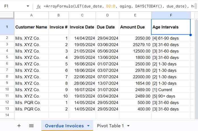
Now, in column F, we will assign the age intervals using an array formula. Enter the following formula in cell F1:
=ArrayFormula(LET(
   due_date, D2:D,
   aging, DAYS(TODAY(), due_date),
   header, "Age Intervals",
   VSTACK(
      header,
      IF(due_date="", ,
         IF(aging<1, "[1] Current",
            IF(aging<31, "[2] 1-30 days",
               IF(aging<61, "[3] 31-60 days",
                  IF(aging<91, "[4] 61-90 days", "[5] 90+ days")
               )
            )
         )
      )
   )
))
This is the only formula required in the sheet to create the age analysis using the pivot table.
The formula assigns the aging intervals based on the due date as follows:
- [1] Current: Invoices that are not past due.
- [2] 1-30 days: Invoices that are 1-30 days past due.
- [3] 31-60 days: Invoices that are 31-60 days past due.
- [4] 61-90 days: Invoices that are 61-90 days past due.
- [5] 90+ days: Invoices that are more than 90 days past due.
The numbers in front of each interval ensure that they are sorted in order when we pivot the data.
Note: The formula is a nested IF formula that evaluates the output of the DAYS function (i.e., today’s date minus the due date) to determine the appropriate age bucket and assigns the aging intervals accordingly. Follow the same format without worrying about the complexity of the formula.
Create an Age Analysis Pivot Table
With minimal effort, anyone can create an accounts receivable (AR) age analysis from the prepared data. Here are the steps to follow:
- Select the Data Range:
- Highlight the data range A1:F.
- Insert the Pivot Table:
- Click on Insert > Pivot table > Create to insert a new sheet with a blank pivot table.
- Configure the Pivot Table:
- In the sidebar pivot table editor panel:
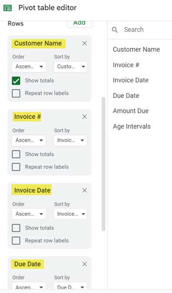
- Drag and drop the fields Customer Name, Invoice #, Invoice Date, and Due Date under Rows.
- Uncheck Show totals for Invoice #, Invoice Date, and Due Date.
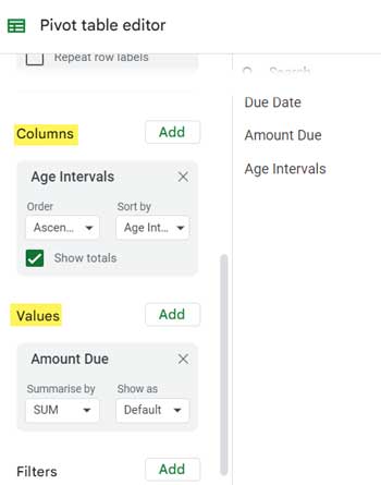
- Drag and drop Age Intervals under the Columns field.
- Drag and drop Amount Due under the Values field.
- Drag and drop Customer Name under Filters, uncheck Blanks, and click OK.
- In the sidebar pivot table editor panel:
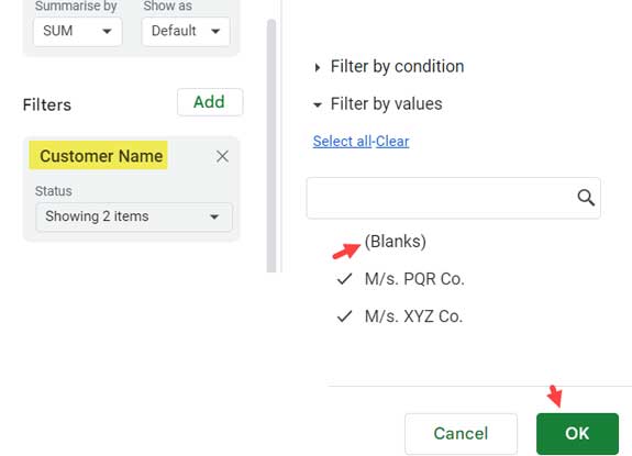
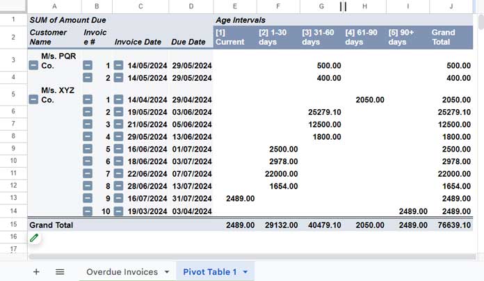
That’s all you need to do. Your AR age analysis report using the pivot table is ready now.
Update and Refresh Your Age Analysis Report
When you add more data, you should take care of a few important things.
In the source sheet, you can enter data in columns A to E. Column F will auto-populate the corresponding age intervals for the new records.
To refresh the age analysis pivot table, follow these steps:
- Hover your mouse pointer over the pivot table report to see the pencil icon.
- Click it to open the pivot table editor panel.
- Click the drop-down under the Filters and click the Select All link.
- Uncheck Blanks.
- Click OK.


You can simplify your formula:
=IF(E2<30,"1. CURRENT",IF(E2<60,"2. 30-60 DAYS",IF(E2<90,"3. 60-90 DAYS",IF(E229,E2<60)(and others like it) because the earlier tests would include those under 30 days.Plus, don't most aging reports do <30, 31-60, 61-90, 91-120, and 121+ so those at 30, 60, 90, and 120 days are explicitly in a single group? Thus:
=IF(E2<30,"1. CURRENT",IF(E2<60,"2. 31-60 DAYS",IF(E2<90,"3. 61-90 DAYS",IF(E2<119,"4. 91-120 DAYS","5. 121 DAYS & ABOVE"))))I’ve updated this tutorial with a new formula and fresh sample data.