Want Excel to automatically display tasks that span multiple days — just like a real project calendar? You’re in the right place. We’ll use Excel formulas to build a smart, fully automated calendar that tracks task durations without VBA or macros.

You’ll also get smart interactive controls to:

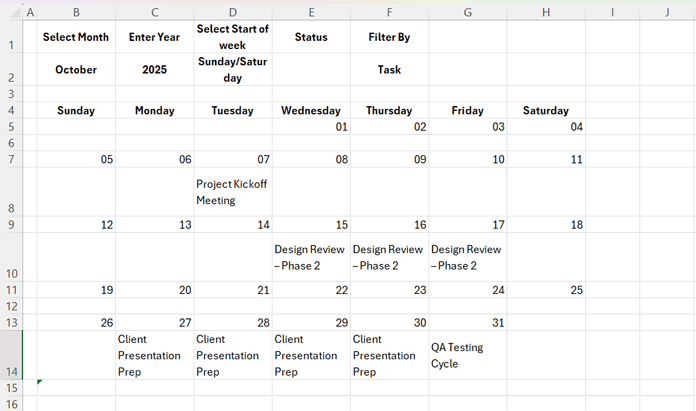
• Select Month
• Enter Year
• Choose Week Start (Sunday or Monday)
• Filter by Status
• Filter by Task or Assigned Person

Your calendar will even highlight today’s date and the current week automatically — updating instantly when you change your selections.

By the end, you’ll have a clean, auto-updating Excel project calendar that’s flexible enough to handle tasks, durations, and team assignments.

Why Build an Excel Calendar with Task Durations?

Most Excel calendars show one-day events. But real projects rarely work that way.

Maybe your design review lasts three days, or your financial audit spans a week. With a traditional calendar, you’d have to manually fill each day. That’s where a smart Excel calendar with task durations saves you time.

It can:

• Automatically fill all dates between each task’s start and end date
• Instantly update when you change the month or year
• Work 100% with formulas — no scripts or coding required

In this tutorial, you’ll learn how to build a dynamic Excel calendar with task durations using formulas like LET, FILTER, and SEQUENCE — no VBA needed.

Let’s get started.

Step 1: Basic Setup for Your Smart Excel Calendar

Let’s start with the basic setup — something most of you will find familiar.

1. Open Microsoft Excel 2021, Excel 365, or later (including Excel 2024).
2. Create a new Blank Workbook.
3. Rename the first sheet to Task Data by double-clicking the sheet tab at the bottom.
4. Add another sheet and name it Calendar View.
5. Save your workbook as Smart Excel Calendar with Task Durations.

That’s it! We’re now ready to prepare the task data and connect it to a live, dynamic calendar.

Step 2: Create the Task Data Table

On the Task Data sheet, enter your project details.

In cells B3:F3, add the following headers:
Task, Start Date, End Date, Assigned To, and Status.

Then, fill in some sample data below the headers:

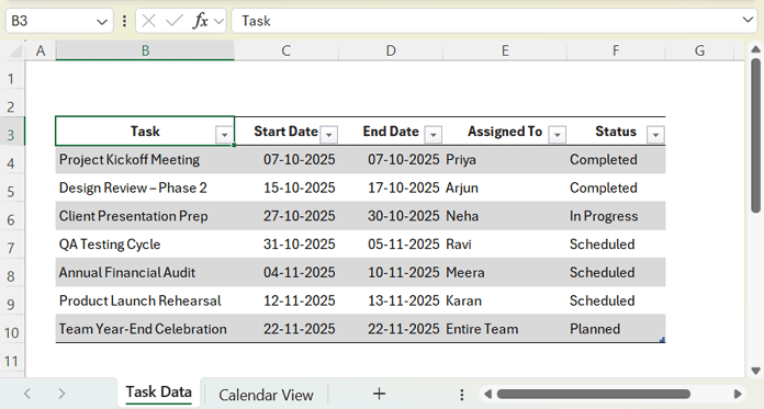
Now, let’s turn this into a proper Excel Table so you can use structured references in formulas — allowing them to automatically expand or shrink as your data grows or changes.

To do that:

1. Select the entire range of your data.
2. Go to Insert → Table.
3. Check the box My table has headers, then click OK.
4. With any cell in the table selected, go to the Table Design tab.
5. In the Table Name field, rename it to Task_Data.

Step 3: Add Smart Controls

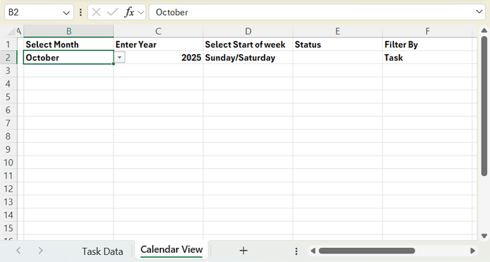
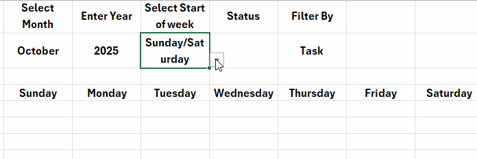
Head to the Calendar View sheet and set up the following labels:

• B1: Select Month
• C1: Enter Year
• D1: Select Start of Week
• E1: Status
• F1: Filter By

Now, you’ll create four drop-down lists in cells B2, D2, E2, and F2.

Month Selector (B2)

1. Select cell B2.
2. Go to Data → Data Validation (under the Data Tools group).
3. In the dialog box, set Allow to List.
4. In the Source field, enter: January,February,March,April,May,June,July,August,September,October,November,December
5. Click OK.

Week Start (D2)

1. Select cell D2.
2. Go to Data → Data Validation → List.
3. In the Source field, enter: Sunday/Saturday,Monday/Sunday
4. Click OK.

Status Filter (E2)

1. Select cell E2.
2. Go to Data → Data Validation → List.
3. In the Source field, enter: Completed,In Progress,Scheduled,Planned
4. Click OK.

Note: Ensure these values exactly match the text used in your “Status” column in the Task_Data table.

Filter By (F2)

1. Select cell F2.
2. Go to Data → Data Validation → List.
3. In the Source field, enter: Task,Person
4. Click OK.

Default Setup Example

Once the drop-downs are ready, set your initial values as follows:

These smart controls will drive your Excel calendar with task durations — letting you easily switch between months, change week-start preferences, and filter the displayed tasks dynamically.

Step 4: Generate the Dynamic Excel Calendar Grid

Now comes the exciting part — building the actual Excel calendar with task durations that automatically adjusts when you change the month, year, or week start.

Add Weekday Headers

In cell B4, enter this formula:

=LET(
  wD, HSTACK("Sunday","Monday","Tuesday","Wednesday","Thursday","Friday","Saturday"),
  IF(D2="Sunday/Saturday",
    CHOOSECOLS(wD, SEQUENCE(7)),
    CHOOSECOLS(wD, SEQUENCE(1, 6, 2), 1)
  )
)

This formula dynamically updates the weekday headers based on the week-start option you select in cell D2.

Here’s what it does:

• wD defines the weekday names from Sunday through Saturday.
• The IF condition checks the drop-down in D2:
  • If it’s Sunday/Saturday, it shows the days in their regular order.
  • If it’s Monday/Sunday, it shifts the order so the week starts on Monday instead.

That means your weekday headers always match your preferred start of the week — automatically!

Create the First Week

Next, in cell B5, enter this formula:

=LET(
  my, DATE(C2, MONTH(B2&1), 1),
  dts, SEQUENCE(1, 7, my-WEEKDAY(my, IF(D2="Sunday/Saturday", 1, 2))+1),
  fnl, dts*(EOMONTH(dts,0)=EOMONTH(my, 0)),
  IF(fnl, fnl, "")
)

Then, format the range B5:H5 as DD (so only the day numbers appear) by going to Home > Format > Format Cells > Number > Custom > Type: DD.

How it works:

• my gets the first date of your selected month and year.
• SEQUENCE generates 7 consecutive dates (one for each day of the week).
• WEEKDAY aligns the start of the week based on your drop-down selection.
• EOMONTH keeps only dates that belong to the selected month, hiding any spillovers from the previous month.
• Finally, IF(fnl, fnl, “”) ensures that blank cells stay empty for a clean layout.

Extend the Calendar

Now let’s expand the calendar for the remaining weeks.
In cell B7, enter this formula:

=LET(
  my, DATE($C$2, MONTH($B$2&1), 1),
  dts, SEQUENCE(1, 7, H5+1),
  fnl, dts*(EOMONTH(dts, 0)=EOMONTH(my, 0)),
  IFERROR(IF(fnl, fnl, ""), "")
)

Copy this formula from cell B7 down every two rows — for example, into B9, B11, B13, and B15. Format these rows as DD as you did earlier.

What it does:

• my identifies the first day of the selected month and year.
• dts generates a new week starting right after the previous one.
• EOMONTH filters out any dates outside the current month.
• IFERROR removes unnecessary error messages, keeping your calendar neat.

And that’s it — your base calendar grid is ready!

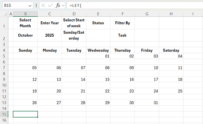
Whenever you change the month, year, or week start, the entire calendar updates instantly. This forms the core of your smart Excel calendar with task durations, ready to display live task data in the next step.

Step 5: Link Task Data Table to the Calendar View

Now we’ll make each date cell display the corresponding tasks (or assigned team members).

In B6, enter:

=IFERROR(
  IF(B5="", "", TEXTJOIN(CHAR(10), TRUE,
    FILTER(
      IF($F$2="Task", Task_Data[Task], Task_Data[Assigned To]),
      (Task_Data[Start Date]<=B5)*(Task_Data[End Date]>=B5)*
      (IFERROR(SEARCH($E$2, IF(Task_Data[Status]="","-", Task_Data[Status])), 0))
    )
  )), ""
)

Copy this formula from cell B6 to:
C6:H6, B8:H8, B10:H10, B12:H12, B14:H14, B16:H16

Then, select B6:H16 and apply Wrap Text from the Home tab.
Next, select rows 6 to 16, and double-click on any row boundary to automatically adjust the height so all text fits neatly within each cell.

How It Works

• TEXTJOIN(CHAR(10)) → Joins multiple tasks in one cell, separated by line breaks.
• FILTER() → Extracts all tasks or assignees (as per your selection in F2) that overlap the specific date.
• $F$2=”Task” → Switches between viewing Task names or Assigned people.
• SEARCH($E$2, Status) → Applies the optional status filter.
• IFERROR() → Keeps cells blank when no matching tasks are found.

Each cell in your calendar now automatically displays every task (or assignee, if F2 is set to Person) that’s active on that day.
To view tasks with a specific status, choose the status in E2 — or leave E2 blank to see all statuses.

Step 6: Add Focus to Today and the Current Week

We’ve now created a smart Excel calendar that displays task durations. Let’s highlight today’s date and the current week to bring focus.

Highlight the Current Week

1. Select the range B5:H16.
2. Go to Home → Conditional Formatting → New Rule → Use a formula to determine which cells to format.
3. Enter the following formula:
   =LET(return_type, IF($D$2="Sunday/Saturday", 1, 2), OR(IFERROR(WEEKNUM(B4, return_type), "")=WEEKNUM(TODAY(), return_type), IFERROR(WEEKNUM(B5, return_type), "")=WEEKNUM(TODAY(), return_type)))
4. Click Format → Fill, and choose a Baby Blue color.

Note:
The formula checks the value in D2 to decide how the week numbering is calculated.

• If D2 is set to “Sunday/Saturday”, the week starts on Sunday.
• Otherwise, it starts on Monday.

Highlight Today’s Date

1. Repeat the same steps to create a new rule.
2. Enter this formula: =OR(B5=TODAY(), B4=TODAY())
3. Set the Fill color to Deep Sky Blue and the Font color to White.

Your calendar now visually highlights the current week in Baby Blue and today’s date in Deep Sky Blue — making it easy to focus on what’s happening right now.

Step 7: Add Conditional Borders

Instead of manually adding borders to the calendar grid, let’s take a more intuitive approach using conditional formatting.
(Of course, this step is optional — you can always apply borders manually.)

The advantage of this method is that the borders will automatically adjust based on the selected month and year — leaving cells outside the current month border-free.

Step 1: Add Top, Left, and Right Borders to the Date Rows

1. Select the range B5:H16.
2. Go to Home → Conditional Formatting → New Rule → Use a formula to determine which cells to format.
3. Enter the following formula: =IFERROR(YEAR(B5)=$C$2,"")
4. Click Format → Border, and apply Top, Left, and Right borders.

Step 2: Add Bottom, Left, and Right Borders to the Data Rows

1. Add another new conditional formatting rule with this formula: =IFERROR(YEAR(B4)=$C$2,"")
2. Apply Left, Right, and Bottom borders.

Final Touch and Layout Adjustment

Finally, adjust the row heights and column widths manually to achieve the perfect layout.
Also, turn off the gridlines for a cleaner look.

Your calendar grid will now automatically display borders only for the dates that belong to the selected month and year, keeping the empty cells neat and visually clear.

FAQ: Smart Excel Calendar with Task Durations

1. Will this work in older versions of Excel (like 2019 or 2016)?
This tutorial uses modern Excel functions like LET, FILTER, and SEQUENCE, which are available in Excel 2021, Excel 365, and later (including Excel 2024).
Older versions such as Excel 2019 or 2016 don’t support these functions, so the calendar won’t work as intended there.

2. The calendar looks empty — what could be wrong?
If no tasks appear:

• Check that your Task_Data table name matches exactly.
• Ensure your Start Date and End Date columns contain valid Excel date values (not text).
• Verify that E2 (Status) is blank or matches one of the Status values in your data.

3. How do I reset the calendar for a new year or project?
Simply change the Month and Year in B2 and C2.
The entire calendar, tasks, and highlights will update automatically.

4. How can I print or share the calendar?
Go to Page Layout → Print Area → Set Print Area, and then adjust scaling to “Fit to One Page.”
Alternatively, export it as a PDF for easy sharing with your team.

5. Can this calendar be used for resource planning or leave tracking?
Yes. By switching F2 to Person, you can see each team member’s active tasks on a given day — making it ideal for leave tracking, shift planning, or resource allocation.

Final Thoughts on Building a Smart Excel Calendar with Task Durations

And there you have it — your own smart Excel calendar with task durations that requires no VBA or macros.

What started as a simple date grid is now a fully dynamic project tracker that automatically shows which tasks are active on each day, highlights deadlines, and adapts instantly to your selected filters.

It’s perfect for project management, audits, marketing plans, event scheduling, or any scenario where you need to visualize multi-day timelines right inside Excel.

Try it out, customize it for your team, and see how easily Excel can become your most powerful planning tool.

Download the Free Template:

Download the Smart Excel Calendar Template

(Click the button above to get the ready-to-use file and explore all features.)

Tip:
If you only need to plot single-day events, check out my tutorial —
Populate Dynamic Calendar from a Table in Excel