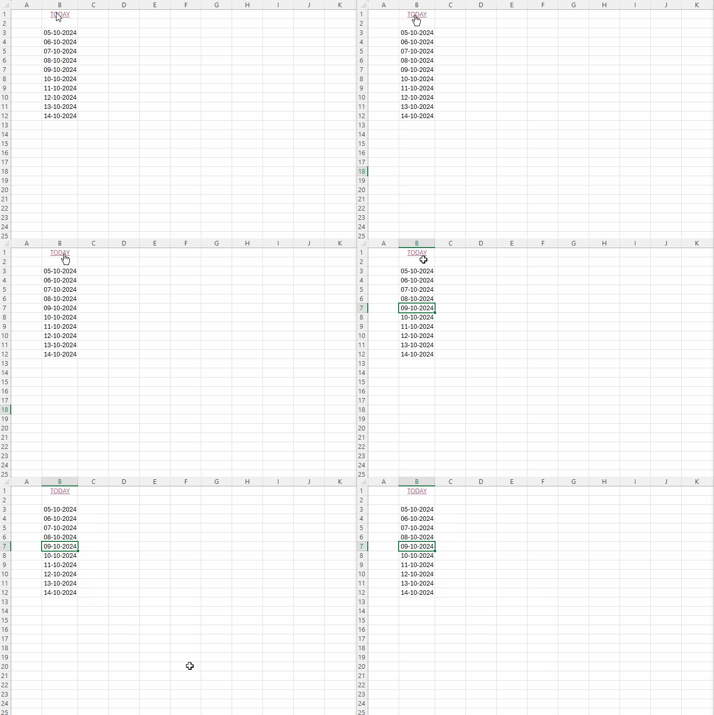
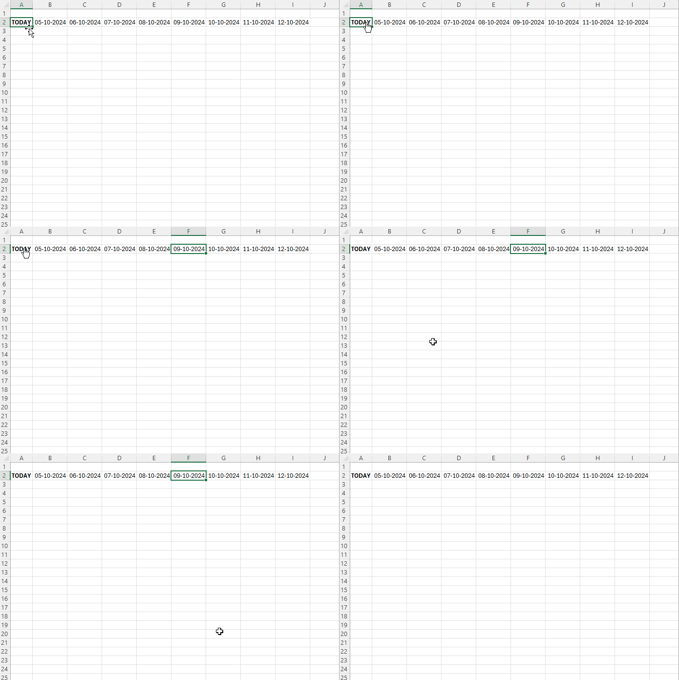
We can create a hyperlink to quickly jump to the first occurrence of the current date in a row or column in Excel. We will use MATCH, INDEX, CELL, and HYPERLINK functions to achieve this. If your version of Excel supports the XMATCH function, you can also create a hyperlink to jump to the last occurrence of the current date.
Example Scenario
Assume you have dates in the range B2:B100, and you want a link in cell B1 with the label “Today.” When you click this link, it will take you to the first occurrence of the current date in B2:B100.
The same approach can also be applied to jump to the current date across rows in Excel.
The Logic Behind Jumping to the Current Date Cell in Excel
Assume you want to jump to cell B50; you can use the following formula in any cell:
=HYPERLINK("#B50", "LINK LABEL")You can replace “LINK LABEL” with any text you want for the hyperlink label.
To dynamically jump to the current date cell, the process involves finding the cell reference that contains today’s date and then using that reference within the HYPERLINK function.
Formula and Explanation
The formula differs depending on whether you are working with columns or rows. To find the current date in a column and create a clickable link that jumps to that cell, use the following formula:
=HYPERLINK("#"&CELL("ADDRESS", INDEX(range, MATCH(TODAY(), range, 0))), "TODAY")In this formula, replace range with the actual range where you want to locate today’s date.
To find today’s date in a row and create a clickable link that jumps to that date, use this formula:
=HYPERLINK("#"&CELL("ADDRESS", INDEX(range, 0, MATCH(TODAY(), range, 0))), "TODAY")Again, replace range with the specific range you want to search for today’s date.
Example 1 (Column Formula):
If you enter the following formula in cell B1, it will create a link with the label “TODAY.” When clicked, the link will jump to cell B7 if that cell contains today’s date:
=HYPERLINK("#"&CELL("ADDRESS", INDEX(B2:B100, MATCH(TODAY(), B2:B100, 0))), "TODAY")
Example 2 (Row Formula):
Similarly, if you enter the following formula in cell A2, it will create a link with the label “TODAY.” When clicked, it will jump to cell F2 if that cell contains today’s date:
=HYPERLINK("#"&CELL("ADDRESS", INDEX(B2:Z2, 0, MATCH(TODAY(), B2:Z2, 0))), "TODAY")
Formula Explanation
Let’s break down the column formula for better understanding:
MATCH(TODAY(), range, 0)- This finds the relative position of today’s date within the specified range.
INDEX(B2:B100, …)- This returns the value (or cell reference) in the range B2:B100 based on the row number returned by the MATCH function.
CELL("ADDRESS", …)- This returns the address (in text form) of the cell found by the INDEX function.
"#"&…- The “#” symbol is combined with the cell address to form the
link_locationfor the HYPERLINK function.
Finally, the formula:
=HYPERLINK(link_location, friendly_label)The link_location is the cell address prefixed by “#”, and the friendly_label is the text displayed for the link (in this case, “TODAY”).
Key Difference for Rows:
The only difference when working with rows is in the INDEX function. Instead of a row offset (used for columns), the formula uses a column offset to find the correct date.
XLOOKUP Enhancement: Jump to the Last Occurrence of the Current Date
If your version of Excel supports XLOOKUP, you can try this additional tip.
Sometimes your rows or columns contain multiple occurrences of a date, and the last occurrence may represent the most recent value.
If you want to jump to the last occurrence of today’s date in a column or row, replace the MATCH function with the following XMATCH:
XMATCH(TODAY(), range, 0, -1)The -1 in XMATCH tells Excel to search in reverse, returning the last occurrence of today’s date in the specified range.


