Finding Most Frequent Text in Excel with Dynamic Array Formulas

Looking to identify the most frequently occurring text in Excel? You can do this easily using dynamic array formulas. With this approach, similar to MODE.MULT, if there’s a tie, the formula will return all tied values.

As a quick note, MODE.MULT is an Excel function that returns the most frequently occurring numeric values in a dataset. Here, we’ll use some techniques to adapt it for text data.

Table of Contents

Generic Formula

Here’s a general formula that you can use to find the most common text in a specified range in Excel:

=LET(
   range, TOCOL(cell_range, 1),
   val, IFNA(XMATCH(range, range),0),
   modeN, MODE.MULT(val),
   XLOOKUP(modeN, val, range)
)

Where:

cell_range: Replace this with the actual range you want to analyze, such as A1:A100.

This formula will return the text that appears most frequently. If there is a tie, it will return all tied text values.

Example of How It Works

If “apple” appears 51 times and “orange” appears 49 times, the formula returns “apple.”

If both “apple” and “orange” appear 50 times each, it will return both “apple” and “orange” as results.

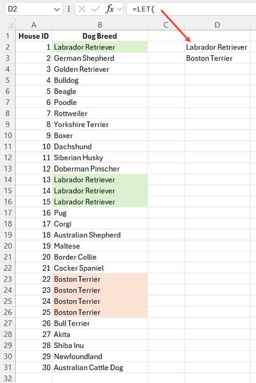
Example: Finding the Most Commonly Occurring Dog Breeds

Let’s say you conducted a survey where column A contains house numbers and column B lists dog breeds in each house. Your data range is A1:B31, with headers in A1:B1.

To find the most common dog breed(s) in this survey, use the following formula:

=LET(
   range, TOCOL(B2:B31, 1),
   val, IFNA(XMATCH(range, range),0),
   modeN, MODE.MULT(val),
   XLOOKUP(modeN, val, range)
)

For example, if “Labrador Retriever” and “Boston Terrier” each appear four times and no other dog breed appears more frequently, the formula will return both breeds.

Counting the Most Frequently Occurring Text in Excel

To determine how many times each breed appears, you can use the COUNTIF function with the results. I’ll cover this after breaking down the formula above.

Formula Break-Down

Let’s go over each part of the formula to understand how it works.

Step 1: Find Relative Positions with XMATCH

=IFNA(XMATCH(B2:B31, B2:B31), 0)

XMATCH in Excel returns the relative position of each item within the range. If a breed appears multiple times, each occurrence will share the same relative position.

Example: If “Labrador Retriever” is the first value in cell B2, XMATCH assigns it position 1 wherever it appears in B2:B31.

Step 2: Get the Most Frequent Position with MODE.MULT

=MODE.MULT(IFNA(XMATCH(B2:B31, B2:B31), 0))

MODE.MULT calculates the most frequently occurring relative positions in the dataset returned by the formula in step 1, allowing us to identify any tied values.

Step 3: Look Up Most Frequent Text with XLOOKUP

=XLOOKUP(
   MODE.MULT(IFNA(XMATCH(B2:B31, B2:B31), 0)),  
   IFNA(XMATCH(B2:B31, B2:B31), 0), 
   B2:B31
)

Using MODE.MULT as the search key, XLOOKUP retrieves the text values associated with the most frequent relative positions in B2:B31.

This formula can be simplified conceptually as:

=XLOOKUP(
   step_2_formula,  
   step_1_formula, 
   B2:B31
)

Step 4: Using LET for Efficiency

To make the formula cleaner and more readable, we can use the LET function to assign names to parts of the formula:

Syntax of LET:

=LET(name1, value1, calculation_or_name2, [value2, calculation_or_name3…])

In our final formula that returns the most frequent text values, the arguments are:

name1: range
- value1: TOCOL(B2:B31, 1) — TOCOL removes empty cells, if any.
name2: val
- value2: IFNA(XMATCH(range, range), 0) — the formula that finds relative positions in the range.
name3: modeN
- value3: MODE.MULT(val) — the formula that finds the most frequently occurring positions.
calculation: XLOOKUP(modeN, val, range)

This final formula is now simpler and easier to understand:

=LET(
   range, TOCOL(B2:B31, 1),
   val, IFNA(XMATCH(range, range), 0),
   modeN, MODE.MULT(val),
   XLOOKUP(modeN, val, range)
)

Using LET helps keep the formula organized and reduces repetitive calculations, making it more efficient and readable.

Additional Tip: Counting the Most Frequently Occurring Text

To count how many times each of the most frequent texts appears, use COUNTIF with the results.

=COUNTIF(B2:B31, D2)

Here:

B2:B31 is the range with the original data.
D2 is the cell containing one of the most frequent text strings returned by the formula.