


Creating a table of contents in Google Sheets is simple, but understanding its spreadsheet purpose is vital.
In traditional printed documents, a table of contents offers an overview of the content. In digital documents like Word and Docs, it serves the additional function of enabling readers to navigate to specific sections within the document.
There are primarily two types of tables of contents in spreadsheets, each serving a specific purpose:
- Navigating to Different Rows or Columns (Sections) Within the Sheet.
- Navigating to Different Sheets Within the File.
Navigating to different sheets is facilitated through the “All Sheets” button, located at the bottom left next to the + button. This button displays all sheets in the workbook (file), simplifying navigation. However, there are instances where a dedicated table of contents in Google Sheets proves advantageous.
Imagine a file with 25 sheets, where 10 are main sheets and the rest serve as helper sheets or contain draft input. In such cases, using the All Sheets option might become cumbersome.
To address this, you can create a table of contents on the first sheet that includes only the main sheets, providing users with a streamlined navigation option. Additionally, you can incorporate relevant information about each sheet, offering users an overview of the content.
Now, let’s explore the steps to create a table of contents in Google Sheets.
Creating a Google Sheets Table of Contents with Sheet Names
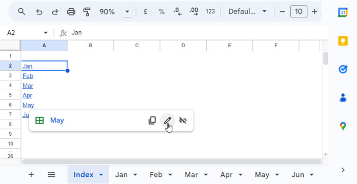
In the following example, I have 6 sheets named Jan, Feb, Mar, Apr, May, and Jun in a Google Sheets file. To create a table of contents in this file, follow the steps below:
- Click the + (Add Sheet) button at the bottom left corner to create a new sheet.
- Right-click on the newly created sheet’s tab name and click Rename to rename it to “Index,” “TOC,” or any preferred name.
- Select cell A2 in that sheet and click on “Insert” > “Link.”
- In the dialog box that appears (please see the GIF below), click on “Sheets and named ranges” to view all sheet names in your file.
- Click on “Jan” and press the Enter key.
Repeat the process for cells A3, A4, A5, A6, and A7, inserting the respective sheet names. Your table of contents is now ready.
Now, when you click on the title in the table of contents, it will take you to the relevant sheet in the file at the active cell where you were last in that sheet.
If you want customized names to appear instead of the original sheet names, follow these steps:
- Hover your mouse pointer over the sheet name in the table of contents.
- Click on the pencil icon and replace the sheet name with the text you want.
Creating a Table of Contents with Links to Cells in Google Sheets
In a very large spreadsheet, the above link to sheets may not be effective for navigating to specific sections (tables) within the same sheet. These links are primarily designed for transitioning between separate sheets. To efficiently navigate to specific sections within a single sheet, it is necessary to obtain the cell URLs. Here’s how to achieve this:
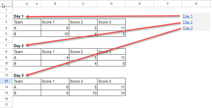
In the following example, I have three sections: “Day 1,” “Day 2,” and “Day 3,” starting in cells D2, D7, and D12, respectively.
Here’s how to link to them in a table of contents:
- Enter “Day 1,” “Day 2,” and “Day 3” in the cell range G2:G4. You do not need to stick with the same names. Also, you can create the table of contents in a different sheet other than the one the tables contain.
- To get the link to “Day 1,” right-click on cell A2 and click on “View more cell actions” > “Get link to this cell.”
- Go to cell G2 in the table of contents and click on “Insert” > “Link.” Paste the copied URL in the search field and click Apply.
- To get the link to “Day 2,” right-click on cell A7 and click on “View more cell actions” > “Get link to this cell.”
- Go to cell G3 in the table of contents and click on “Insert” > “Link.” Paste the copied URL in the search field and click Apply.
This way, you can create a table of contents using cell URLs in Google Sheets.
Related: Dynamic Cell Reference in Table of Contents in Google Sheets.
Conclusion
In the above discussion, I’ve presented two distinct methods for creating a table of contents in Google Sheets. The first method is designed for navigating to different sheets, while the second is tailored for navigating to different sections within a sheet.
Unlike document editors, Google Sheets allows you to leverage formulas to enhance the table of contents, especially with the first approach that utilizes sheet names as the table of contents list.
For instance, in cell B2, you can use the formula =INDIRECT(A2&"!A1:B1") to retrieve values from cells A1:B1 in the “Jan” sheet. Simply copy and paste the B2 formula into B3 to obtain values from the same cells in the “Feb” sheet.
That concludes our discussion. Thank you for staying with us. Enjoy!
The problem with this method is that if the referenced cell changes (e.g., B100 to B110), the link will not update to the new cell, and you’ll have to continuously update the link manually.
I wish there was a way to maintain the reference dynamically after the initial setup.
Hi, Anthony Escribens,
I have a solution to this. I’ll post it separately or update the above post soon.
I’ll update you below.
Thanks for your valuable feedback.
Hi, Anthony Escribens,
This tutorial may help – Dynamic Reference in Table of Contents in Google Sheets.
Thanks for your advice! I learn a lot from your posts.
This is a time-consuming way to do it if you’re looking to link to the whole sheet. Instead, just Right Click > Insert Link > Click in the Link field > Sheets in this spreadsheet > select which sheet
Hi, Andrew,
I understand that. Updated the post.
Thanks.