How to Use VLOOKUP with Multiple Criteria in Google Sheets [Solved]

First of all, let me clarify one thing. VLOOKUP with multiple criteria is possible in Google Sheets!

There are two aspects to the usage of the Vlookup with multiple criteria in Google Sheets. Let me illustrate the same.

1. Vlookup multiple criteria from a single column:

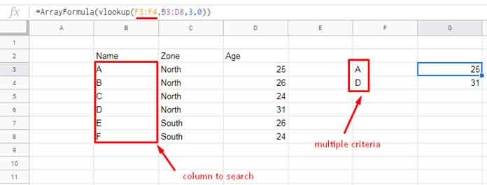
Vlookup multiple conditions - single column

If you are looking for Vlookup formula with more than one criterion from the first column, find the details here – How to Use Vlookup to Return An Array Result in Google Sheets.

2. Vlookup multiple criteria from multiple columns: I am going to explain this topic in this article in detail.

Vlookup multiple conditions - multiple columns

In this scenario, there are two methods that we can follow to deal with 2 or more criteria or also called search keys in VLOOKUP usage in Google Doc Spreadsheets.

Examples and Different Vlookup Approaches

I am using two criteria here in this example. Also, the tips are included to use three or more criteria as shown below.

Google Sheets VLOOKUP function with multiple criteria Usage

Here are the two approaches to deal with multiple criteria in the VLOOKUP formula.

By adding an additional column (helper column) to your dataset – Simple Approach.
Without adding any additional columns or modifications. But by using a virtual helper column (no physical helper column) with the Vlookup formula and also using ArrayFormula – Advanced Vlookup Use and Recommended.

The Simple Approach to Vlookup with Multiple Criteria in Google Sheets

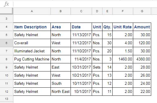
Here is my Sample Data. You can replicate this data on your sheet to follow this tutorial.

Sample Date for Vlookup with Multiple Criteria

I hope you may already know how to use the VLOOKUP formula in Google Doc Spreadsheet. Here is a simple example.

=vlookup("Safety Helmet",A5:G12,7,0)

The above VLOOKUP formula searches the criterion or search_key “Safety Helmet” in the first column of the range A5:G12, i.e. column A, and returns the corresponding value from column index 7, i.e. column G.

Above I’ve used the criteria directly within the formula. When you refer the criteria or search key to a cell, it will be as below.

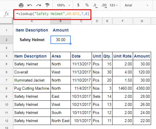
In the above example, VLOOKUP searches only one criterion that is “Safety Helmet” in the first column.

Now I want VLOOKUP to lookup two criteria. The columns to search are the first two columns. How to do that?

Here is our simple approach that involves a physical helper column.

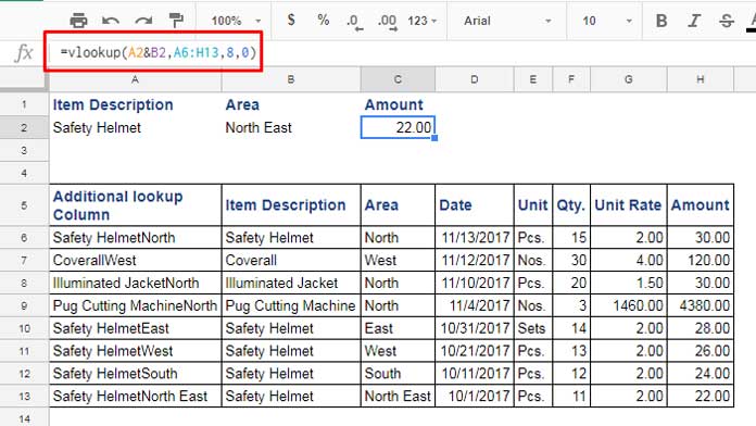
VLOOKUP formula with Multiple Criteria - Simple Approach

See the above example. Here there are two criteria that Vlookup has to search. What are they?

Criterion # 1 is in cell A2, i.e., “Safety Helmet” and the criterion # 2 is “North East” (in cell B2).

To solve this, I have added an additional column labeled as “Additional lookup Column” in our data.

It’s the present column A. This column contains the joined/combined cell values from columns B and C.

Then in our VLOOKUP formula, I have combined criterion from cell A2 and B2. Hope you’ve got this idea.

In Google Sheets, there is a better solution. Without inserting any additional column you can use VLOOKUP in Google Sheets for multiple criteria VLOOKUP.

VLOOKUP with Multiple Criteria in Google Sheets Using ArrayFormula

This is the recommended method to deal with multiple criteria in Google Sheets.

Before going to this trick, I recommend you to go through our usage tips of ArrayFormula, IFERROR, and Curly Braces then come back here. Because I am going to nest all these formulas with VLOOKUP.

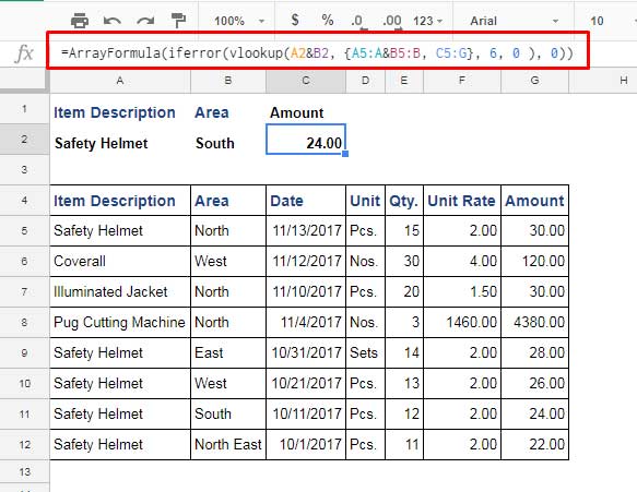
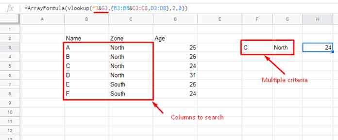
VLOOKUP with Multiple Criteria in Google Sheets using Array

The above is the example of multiple criteria usage with Array (Array Formula and Curly Braces) and Vlookup combination in Google Sheets.

I will explain this formula so that you can use it in any other similar case.

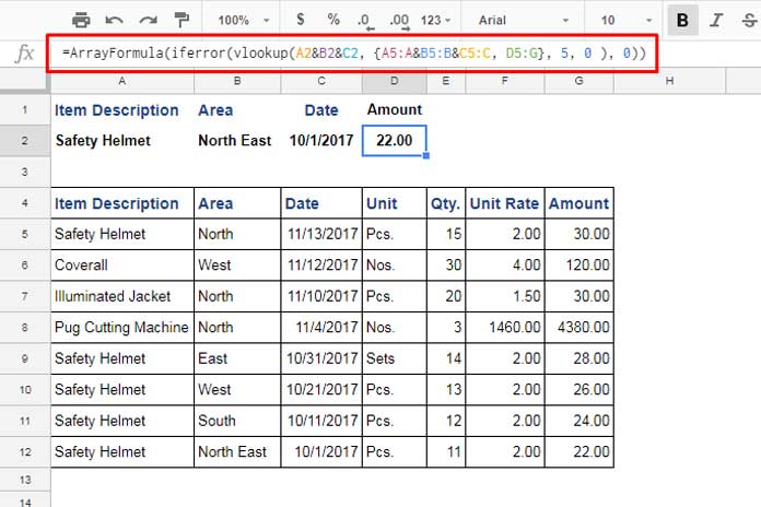
=ARRAYFORMULA(IFERROR(VLOOKUP(A2&B2, {A5:A&B5:B, C5:G}, 6, 0 ), 0))

Formula Explanation Part

Step 1:

VLOOKUP(A2&B2

Here I’ve joined the two criteria from cell A2 and B2.

Step 2:

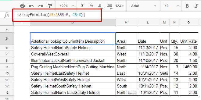
{A5:A&B5:B, C5:G}

In order to understand this part, you should just apply this as below in any cell.

=ARRAYFORMULA({A5:A&B5:B, C5:G})

It will populate the data as below which is our lookup range.

Hope you now understand how to use VLOOKUP with multiple criteria in Google Sheets.

The above example is with two criteria. When there are more than two criteria, you can modify the formula as below.

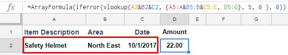
=ARRAYFORMULA(IFERROR(VLOOKUP(A2&B2&C2, {A5:A&B5:B&C5:C, D5:G}, 5, 0 ), 0))

Here my criteria are as below. I’ve included a date also with other two criteria.

VLOOKUP with three criteria in Google Sheets

Thus you can develop the VLOOKUP formula with multiple criteria or conditions.

Additional Vlookup Resources:

39 COMMENTS

Thanasis May 1, 2022 At 5:42 pm

Hello, thank you very much for this extensive coverage of this topic. It is priceless.

I am trying the example with the multiple criteria I can’t get it to work. I am posting the copy that is not working,

– link removed by admin –

Greetings

- Prashanth May 2, 2022 At 3:29 pm
  
  Hi, Thanasis,
  
  The issue lies in the IFERROR part.
  
  Syntax: IFERROR(value, [value_if_error])
  
  In value_if_error, you have put a space and 0 instead of 0. Just correct that.
  
Andrey January 29, 2022 At 5:21 pm

Hi Prashanth,

Help me. Please give me a hint on how to do it.

I need to calculate column B/F under the condition that the dates must match.

An example highlighted in yellow: B15/F4

— link removed by admin —
(with editing rights)

- Prashanth January 31, 2022 At 11:18 am
  
  Hi, Andrey,
  
  You were looking for the correct function. We can use VLOOKUP as below.
  
  =ArrayFormula(ifna(vlookup(E2:E;A2:B;2;0)/F2:F))
  
  The IFNA() removes #N/A! errors if any.
  
  - Andrey January 31, 2022 At 7:02 pm
    
    Thank you! You helped me a lot!
    
    May I ask this question?
    
    I need to copy a formula to cells A1, C1, E1, etc. The insertion interval is the same.
    
    The range A10-A20 contains values for formulas.
    
    The formula should take the values as below.
    
    A1 – A10, C1 – A11, E1 – A12, etc.
    
    - Prashanth February 1, 2022 At 11:31 am
      
      Hi, Andrey,
      
      It’s not related to the topic. But I will try to answer.
      
      If you want the formula to copy to A1, B1, and C1, this approach may work – Drag a Formula across But Get the Reference Down in Google Sheets.
      
      But you want to copy to every alternative column. So I have a helper row approach.
      
      Empty row # 2 and insert the below array formula in A2.
      
      =ArrayFormula(if(iseven(column(A1:1)),1/0, transpose(sequence(rows(A10:A20)*2)-sort({sequence(rows(A10:A20)*2); sequence(rows(A10:A20)*2)}))))
      
      In A1, insert the following formula, which you can copy to C1, E1, G1, etc.
      
      =iferror(INDIRECT("A"&10+A2))
      
      - Andrey February 3, 2022 At 1:29 pm
        
        Hi Prashanth,
        
        Where do you need to correct the formula so that the alternation is not only through the column, but let’s say the alternation goes at any interval?
        
        For example, start in column A, copy to column H, then to column O.
        
        What elegant formulas you get!
        
        Thank you very much!
      - Prashanth February 5, 2022 At 10:40 am
        
        Hi, Andrey,
        
        My earlier formula is not flexible enough to address it.
        
        Here is the flexible one. Here I take the liberty to use one more helper cell to control every N, i.e., cell A3.
        
        In cell A3, enter 7 or the number that controls every alternate column.
        
        Replace my earlier formula in cell A2 with the below one.
        
        =ArrayFormula(if( countifs(transpose(flatten(substitute(sequence(rows(A10:A20),1,0), "",SEQUENCE(1,A3)))),transpose(flatten(substitute(sequence(rows(A10:A20),1,0), "",SEQUENCE(1,A3)))),column(indirect("A2:"&address(2,rows(A10:A20)*A3,4))), "<="&column(indirect("A2:"&address(2,rows(A10:A20)*A3,4))))=1, transpose(flatten(substitute(sequence(rows(A10:A20),1,0), "",SEQUENCE(1,A3)))),1/0))
        
        A tutorial that contains the formula explanation is in the pipeline.
bahar January 27, 2021 At 1:07 pm

Hi Prashanth 😊,

how to sum A:A if multiple same models in my sample sheet? the formula is in cell G2.

— URL of the sheet removed by the admin —

- Prashanth January 27, 2021 At 4:52 pm
  
  Hi, Bahar,
  
  Vlookup is not a suitable formula for you.
  
  Your table is like this (range A1:C).
  Model | Date | Price
  AB5479 | 1 Jan 2021 | 100.00
  CD7150 | 1 Jan 2021 | 180.00
  AB5479 | 1 Jan 2021 | 165.00
  
  Criteria (E2:F2):
  AB5479 | 1 Jan 2021
  
  Use the below formula in cell G2.
  
  =sum(filter(C:C,A:A=E2,B:B=F2))
  
  If you enter more criteria below E2:F2, then you should drag the above formula down.
  
  But you can replace the above formula with the below Sumif array formula in cell G2 which will automatically expand down.
  
  =ArrayFormula(if(len(E2:E),(sumif(A:A&B:B,E2:E&F2:F,C:C)),))
  
  Both the formulas entered in your sheet.
  
Manisahhh December 30, 2019 At 1:21 pm

Hi Prashanth 🙂

Based on your examples, is it possible to use Vlookup with single criteria (“Safety Helmet”) & return all of the matching details?

For example, return all Safety Helmet details in each row. (in form of a table)

ITEM | AREA | AMOUNT
Safety Helmet | North | 70.00
Safety Helmet | West | 80.00
Safety Helmet | East | 75.00

Thank you !!

- Prashanth December 30, 2019 At 5:02 pm
  
  Nope! For that use Filter or Query.
  
  Assume the dataset is in the range A1:C.
  
  Filter:
  
  =filter(A1:C,A1:A="Safety Helmet")
  
  Query:
  
  =query(A1:C,"Select * where A='Safety Helmet'")
  
  See my function guide to learn these two and other popular/useful Google Sheets functions.
  
  - Manisahhh December 31, 2019 At 6:54 am
    
    Thank you so much !! It works 🙂
    
Irina April 13, 2019 At 7:37 pm

Hi, thanks for this. I presume this would not work with 2 drop downs? I’m trying to apply the same method but getting an error.

- Prashanth April 14, 2019 At 9:20 am
  
  Hi, Irina,
  
  Can you please replicate the error on a demo sheet and share it with me here?
  
Brosserg January 11, 2019 At 12:40 am

OK so I used my USA locale Sheet with your formula then when I changed it’s locale to France it auto adjusted my formula to this : =ArrayFormula(IFERROR(VLOOKUP(A2:A&B2:B; {E1:E&F1:F\ G1:G}; 2; 0 ); 0))

So it changed “;” to a “\” and I never would have guessed that.

- Prashanth January 11, 2019 At 8:55 am
  
  Hi, Brosserg,
  
  I guess the formula is working now.
  
  See this supporting tutorial.
  
  How to Change a Non-Regional Google Sheets Formula.
  
  Best,
  
Kay November 15, 2018 At 11:34 pm

Hi,

I need something like this but combined with an importrange function.

Basically, I have one list with extensive data (tour data of artists) and I need to return just some of the sales-figures into another sheet.

So, in File Marketing it should pull the value of File Sales, column I IF in File Sales the artist name is the same as in Column A in File Marketing. So far, that works with Vlookup & importrange.

BUT – there is a second criterion that needs to match in both sheets in order to pull the correct value.

So only if in File Marketing the column A (Artist name) AND column B (date) are the same as in the respective artist & date columns in sheet Sales, I want the value of column I in sales pulled into sheet marketing.

So far, this is the formula that works:

=vlookup(A2:A, Importrange("URL","'Presales '18'!D2:I"),6,0)

with your tutorial, I tried to modify it into

=ARRAYFORMUL(iferror(vlookup(A2:A&B2:B,{Importrange("URL","'Presales '18'!D2:d&G2:g,h2:I")},2,0)))

but nothing shows up – but also no error or parse warning.

I guess the area and column index is wrong, but I don’t know how?

Thanks a lot, Kay

- Prashanth November 16, 2018 At 9:30 am
  
  Hi, Kay,
  
  Let me cross check your question and I will possibly come back with a tutorial that addresses it by today itself. I will post the link here then.
  
  Thanks.
  
- Prashanth November 16, 2018 At 3:14 pm
  
  Hi, Kay,
  
  As promised, here is the tutorial.
  
  How to Vlookup Importrange in Google Sheets [Formula Examples]
  
  You can use either Query or Vlookup with Importrange to get your expecting result.
  
Samah Sohrab November 3, 2018 At 12:16 am

Hi,

Is there a way to not require creating a new combined column, “Additional lookup Column”?

Thanks

- Prashanth November 3, 2018 At 6:15 am
  
  Hi,
  
  It’s already included in this tutorial. Seems you have missed that.
  
Corissa August 14, 2018 At 8:26 am

Hi –

This information was very helpful for a project I’m working on!

I seem to be having a similar issue as others who have commented. I tried to work through the formula differently based on your responses to them, but I’m still getting “0” as the result & the index was being recognized as part of the range.

Note: Link removed by the admin.

=ArrayFormula(iferror(vlookup(A2&B2, {A6:A11&B6:B11, C6:C11},, 2, 0 ), 0))

I feel like I’m missing something really basic/obvious, but I can’t seem to figure it out. Your help is most appreciated!

- Prashanth August 14, 2018 At 11:55 am
  
  Hi, Corissa,
  The formula in your sheet is;
  =ArrayFormula(iferror(vlookup(A2&B2, {A6:A11&B6:B11, C6:C11},, 2, 0 ), 0))
  It should be like this.
  =ArrayFormula(iferror(vlookup(A2&B2, {A6:A11&B6:B11, C6:C11}, 2, 0 ), 0))
  An extra comma in your formula makes that issue.
  Hope this solves the issue.
  Thanks
  
SWWeatherGuy July 25, 2018 At 11:43 pm

I’m trying to use this formula but not getting the desired result, assuming I’m not misunderstanding something. My formula is written:

=ArrayFormula(IfError(VLookup($B$1 & C2, {$B$11:$B & C$11:C, $A$11:$A}, 1, 0), 0))

B1= An entered value of 1-31 days of the month [current value 24]

C2= A Max result from a list of temperature values for the B1 day of the month =Max(Filter(C$11:C,$B$11:$B =$B$1)) [current value 84.3]

A11: A= A list of four-digit year values ranging from 1995 to 2017

Instead of the corresponding year value from A11: A, the result I’m getting is the “search key” [B1&C2] of 2484.3

What am I not understanding?

- Prashanth July 26, 2018 At 8:07 am
  
  Hi,
  
  The column Index should be 2.
  
  Try this.
  
  =ArrayFormula(IfError(VLookup($B$1 & C2, {$B$11:$B & $C$11:C, $A$11:$A}, 2, 0), 0))
  
  a
  
  - SWWeatherGuy July 26, 2018 At 9:25 pm
    
    That indeed worked, thank you! Can you explain why the column index is 2 in this example?
    
Lubos June 27, 2018 At 9:20 pm

Hi Prashanth,

thanks a lot for the tutorial, but I have two questions:
1, in ARRAY function =ArrayFormula({A5:A&B5:B, C5:G}) to what serves the second argument “C5:G”?

2, could you help me to check my equation here:

https://docs.google.com/spreadsheets/d/1K4H6TlTZNJje8Atdf1AgH42UXQ-aAE2q4qy_kqPCAVI/edit?usp=sharing

Basically, the cell I25 should produce value from column X20 if and only if both D25=O20 and K25=T20

Your simple method 1, would work but requires one more redundant column and 2, I cant make work…

Any help much appreciated

- Prashanth June 28, 2018 At 9:25 am
  
  Hi, Lubos,
  
  I’ve checked your sheet. Here is your formula that I’ve found there.
  
  =ARRAYFORMULA((VLOOKUP(D25&K25,{O20:O23&X20:X23},9)))
  
  And see my working Vlookup formula with multiple criteria.
  
  =ARRAYFORMULA((VLOOKUP(D25&K25,{O20:O23&T20:T23,X20:X23},2)))
  
  The logic is simple.
  
  This combines the search keys
  
  D25&K25
  
  So you should combine the corresponding two columns into one.
  
  O20:O23&T20:T23
  
  Now you have only one column. You want the value to return from another column, i.e. from X20: X23.
  
  The below formula makes a two column array and you want the formula to return the value from the column 2 in this array.
  
  {O20:O23&T20:T23,X20:X23}
  
  So I’ve put the index number 2 in Vlookup.
  
  - Lubos June 28, 2018 At 5:09 pm
    
    Hi Prashanth,
    
    thanks a lot, now I understand:-) I got the idea, but in that particular formula you provided the outcome is incorrect. So I25 returns value “6.625”but it should return value of combined “RS3617xs”&”SYNO_A_20180028” which is X20 “213.6”. Actually is seem that value of cell D25 doesnt affect what I25 returns (if you leave it blank, the value will be still “6.625”, but that thats not correct for vlookup)
    
    Sorry I accidentally posted the same question twice. You can delete the other post.
    
    Thanks a lot!!!
    
    - Prashanth June 29, 2018 At 9:16 am
      
      I am sorry about the typo.
      
      I missed the sort order to put at the end. Here is the corrected one.
      
      =ARRAYFORMULA((VLOOKUP(D25&K25,{O20:O23&T20:T23,X20:X23},2,0)))
      
Tamer June 22, 2018 At 7:19 pm

Thanks.
How do I set the range as a named range to use it in VLookup
I tried setting this =ArrayFormula(iferror(vlookup(D12&C12,{G2:G&H2:H,H2:H},2,False)))
I need to set {G2:G&H2:H,H2:H} as a named range so it does not change when I copy the formula between cells but I am unable to do it.

- Prashanth June 23, 2018 At 3:16 pm
  
  Hi, Tamer,
  
  You can not use named ranges here as the formula combines different colums.
  
John Smith April 27, 2018 At 12:42 pm

Clever method! Thanks.

Kris March 24, 2018 At 2:43 am

Thank you!! Awesome!

Konrad March 6, 2018 At 5:25 pm

=ARRAYFORMULA(iferror(VLOOKUP(M17 & N17; {price!A2:A & price!B2:B ; price!C2:C}; 3; 0);0))

Something like that I tried to set also without additional column. But that didn’t worked. It always gave me the second zero (0) which is in iferror function. And also when I parse through VLOOKUP function after going out from { } that number 3 was still interpreted as `range` instead of `index`

- Prashanth March 6, 2018 At 7:03 pm
  
  Hi Konrad,
  
  I tried your formula on my sheet and it works after little modification.
  
  =ARRAYFORMULA(iferror(VLOOKUP(M17 & N17, {price!A2:A & price!B2:B , price!C2:C}, 2, FALSE),0))
  
  The Column Index is 2 not 3. Also based on your locale settings, please change the comma in my formula to semicolon or vice versa.
  
  Please try this and let me know.
  
  Thanks.
  
  - Hugo May 15, 2018 At 6:57 pm
    
    Hi Konrad,
    
    I’ve got the same problem and I can’t find the solution… It always answer 0 even when I change the index number
    
    =ARRAYFORMULA(iferror(VLOOKUP(pich!C2&pich!C3&pich!C4;{arbo!A2:A & arbo!C2:C & arbo!F2:F;arbo!G2:G};6;false); 0))
    
    - Prashanth May 15, 2018 At 7:48 pm
      
      Hi Hugo,
      
      You have only 4 columns (A, C, F, G) and you can’t use index number 6 in Vlookup.
      
      Thanks.