Unlike most of the functions in Google Doc Spreadsheets, you can learn the VALUE function in Google Sheets even without an example. It’s that much simple. So I am directly going to the purpose and syntax part of the Value Function. Don’t worry, I’ve included enough examples to shed some light on the basic and advanced use of this function.

Purpose of Value Function in Google Sheets

The purpose of value function is to convert a string in any of the number, date or time formats into a number. So that you can use this in calculations in the desired way.

You can convert a number, date or time to plain text from the format menu. So it losses its characteristics and can’t be used in Mathematical Operations. Sometimes you may have imported such converted data on to your spreadsheets.

Syntax:

VALUE(text)

How to Use Value Formula in Google Sheets

Here we can see few basic examples of the use of the Value function.

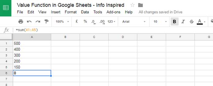
Value function in a column where the numbers formatted as text.

Here as you can see the SUM formula in Cell A6 returns 0 as the formula can’t recognize the numbers.

Here you should know how to use Google Sheets Value function with SUM. A formula like the one below can covert a formatted number in an individual cell to pure number as below.

=Value(A1)

But in our case, it’s an array like A1: A5. Then how to use VALUE function in Google Sheets to covert an array containing text formatted numbers to values?

Here we can make use of the function ARRAYFORMULA. In my personal experience, ARRAYFORMULA is one of the most commonly used functions in Google Sheets. Let’s come back to our topic.

=ArrayFormula(value(A1:A5))

The above formula can convert a range of numbers which is formatted as text, back to numbers. So you can use the below SUM formula in our above example.

=ArrayFormula(sum(value(A1:A5)))

How to use VALUE formula in a column containing Date formatted as text?

Here is the formula to convert a date in text format to number.

=to_date(value(A1))

Yes! Here you should use the date function, to_date, with the VALUE function. Otherwise, the value function would return date value, not the formatted date. Actually, the date value would be sufficient in calculations.

Again here also you should take the use of ArrayFormula to use VALUE formula in an Array.

=ArrayFormula(to_date(value(A1:A2)))

How to use Google Sheets Value formula with Time formatted as Text

See the use of the Google Sheets Value function in Time based calculations. In Date related Value function, we can use to_date function together with Value. But here there is no such option.

I have a time formatted as text in cell A1 as 10:10:45. The Value function can be used to return the value of this time and the result would be like;

0.4241319444

Here there is no option to keep the format of time. But this value is enough in time calculations. For example, the following Value formula in Google Sheets would return the Second from the time value.

=SECOND(0.4241319444)

Result: 45

Advanced Use of Value Function in Google Sheets

You can use the Value function in complex formulas involving Query, Vlookup etc.

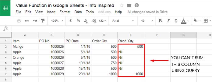
If you use aggregation functions like SUM, AVG in Query in a column that is containing text and numbers, it would return the following type of error.

“Unable to parse query string for Function QUERY parameter 2: AVG_SUM_ONLY_NUMERIC”

Here you can indirectly make use of Google Sheets VALUE function. I am not going to the complete detail. I’ll explain to you how to filter only the number from this Column using Query.

The following formula would only return numbers from the column E. But again it’s formatted as text because we have used a regular expression here.

=QUERY(A1:E7,"select E where E matches '[0-9\-.]+' ",0)

For more details about this formula follow the below link.

Must Read: How to Filter Numbers Only From Mixed Data Column

Now as I’ve told you at the beginning of this tutorial, we should use ArrayFormula when we use VALUE function in an Array. So you can use the below formula to convert the above text formatted numbers returned by Query back to the number.

=ArrayFormula(value(QUERY(A1:E7,"select E where E matches '[0-9\-.]+' ",0)))

The above formula would return the values after filtering out the texts in column E. Now the below Query can return the first four columns that’s column A, B, C, and D.

=QUERY(A1:E7,"select A,B,C,D where E matches '[0-9\-.]+' ",0)

You can join these two Queries with the help of Curly Brackets as below and make use in calculations.

=query({QUERY(A1:E7,"select A,B,C,D where E matches '[0-9\-.]+' ",0),ArrayFormula(value(QUERY(A1:E7,"select E where E matches '[0-9\-.]+' ",0)))},"Select Col1, Sum (Col5) group by Col1")

Conclusion

To become a master in Google Sheets, you should try to learn as much as functions you can regardless of its importance. You can use any functions that seem simple to you in complex combo formulas.

That’s all for now. Hope you have enjoyed!