Sum by Month in Google Sheets Using Combined SUMIF Formula

Here I’m going to share with you a ‘magical’ SUMIF formula to sum by month in Google Sheets. I’m not exaggerating. See what I am going to do.

I am a huge fan of Google Sheets ArrayFormula. So I’m combining ArrayFormula with the SUMIF function to make it a single formula that can sum by month.

The benefit, you need not have to first convert the date to a month in a separate column to sum by month.

Similarly, we can generate month criteria within the formula itself. In other words, you just need to key the formula in just one cell!

Sum by Month in Google Sheets

Before that, I am going to explain to you the simple or you can say the traditional method to sum by month in Google Sheets. Here is that.

Normal Way of Sum by Month in Google Sheets

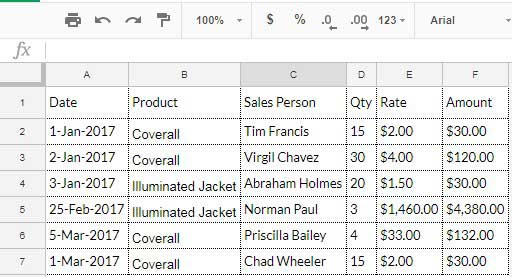
Sample Data:

Steps:

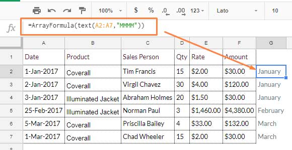
1. First, we should extract the month from the date in a separate column, here column G. To do that use the following TEXT formula in cell G2.

=text(A2,"MMMM")

2. Now in order to expand the formula to below rows, instead of copy and paste, use ArrayFormula.

Just replace the above formula with the following array formula. Now the formula in Cell G2 must be as follows.

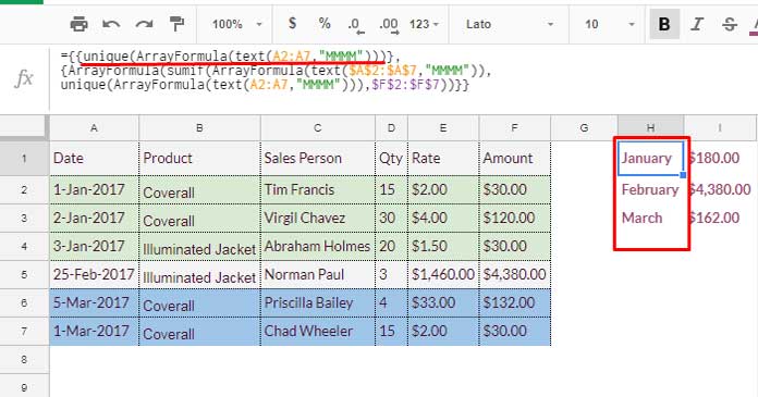
=ArrayFormula(text(A2:A7,"MMMM"))

In order to see the result, please refer to the screenshot below.

extract month from date in Google Sheets

3. So we have converted the date to month. Now we can easily sum by month using SUMIF. But before that one more thing is required.

In Cell H2, use the above same formula but with UNIQUE. This is to generate the criteria for using in SUMIF.

=unique(ArrayFormula(text(A2:A7,"MMMM")))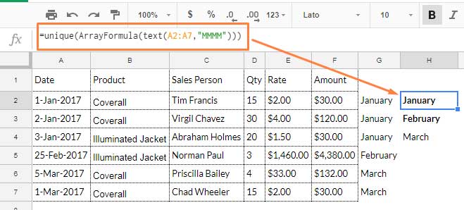

4. Our criteria part is also ready! Now, as usual, we can use SUMIF to sum by month. To do that on Cell I2 apply the below formula.

=sumif($G$2:$G$7,H2,$F$2:$F$7)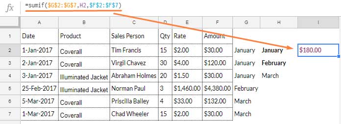

5. You can either copy and paste the above SUMIF formula to the cells down (I3 and I4) or use ArrayFormula in I2 to automatically expand the result. Here is that SUMIF with ArrayFormula Combination.

=ArrayFormula(sumif($G$2:$G$7,$H$2:$H$4,$F$2:$F$7))

Now let us talk about the advanced part. I mean a single formula to do the above all jobs.

Advanced and Flexible Way of Sum by Month in Google Sheets

Here we can combine all the above formulas in one single formula. We are not combining the formulas as it is. There are minor changes like the use of Curly Braces. I will explain to you the difference. See the magical SUMIF formula below.

={{unique(ArrayFormula(text(A2:A7,"MMMM")))},
 {ArrayFormula(sumif(ArrayFormula(text($A$2:$A$7,"MMMM")),
 unique(ArrayFormula(text(A2:A7,"MMMM"))),$F$2:$F$7))}}

I will explain the above combination formula with the help of screenshots.

1. The first part of the formula has nothing to do with the Sum by Month. Refer below image. It’s there because we want to show the corresponding month against the summary value as the prefix.

That means the first part of the underlined formula just returns the unique month names in H1:H3. I’ve used Curly Brackets to separate this with the SUMIF part.

curly brackets with sumif to get criteria on side

Now to the Second Part of the Formula.

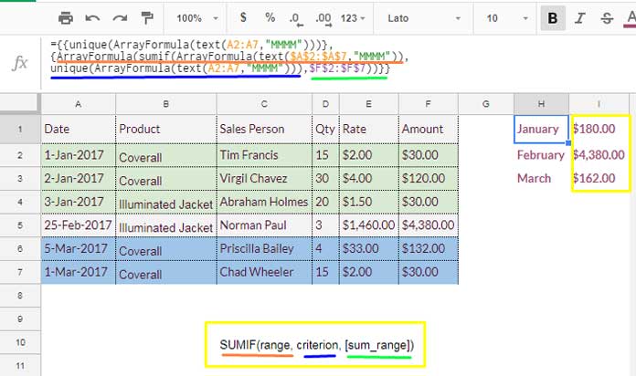
You can see the SUMIF syntax in Cell C10. I’ve just put it there to explain to you the formula in detail. I’ve marked the SUMIF range, criterion, and the Sum range in the formula bar.

The SUMIF(range, is the same formula under point # 2 under the title “Normal Way of Sum by Month in Google Sheets”. Also, Criterion is the same formula under point #3 there. The Sum range is the range from the original data range.

Finally, you can shorten the above formula. We only need one ArrayFormula at the beginning.

Shortened Sumif Array Formula to Sum by Month in Google Sheets:

=ArrayFormula({{unique(text(A2:A7,"MMMM"))},
 {sumif(text(A2:A7,"MMMM"),
 unique(text(A2:A7,"MMMM")),F2:F7)}})

Update Dated 5-Oct-2019 Based on User Feedbacks

How to Include Infinite/Open Ranges in Sumif

I have gone through user comments and could understand two issues they are facing.

How to use an open range like A2:A instead of using a limited range like A2:A7 in the formula.
A Sumif formula to sum by month and year.

I am going to address both the issues here.

Open Range in Sumif Sum by Month Formula

First of all, let’s see what happens when we use open ranges in the above Sumif shortened array formula.

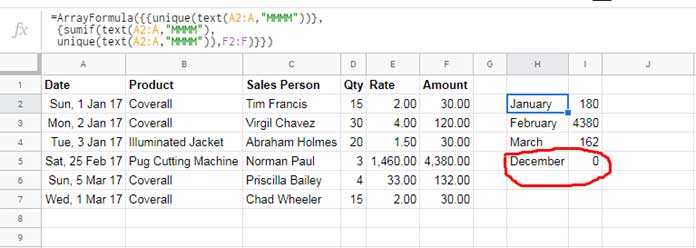
Even though there are no dates in column A that falls in December, the Sumif sum by month formula returns a December month summary row in the output!

This is because of the use of the Text function. Did you try using a blank cell as the reference in Text formula to format a date to month text? For example, in our above Sumif example, the cell A8 is blank. Just try this formula.

=text(A8,"MMMM")

It would return “December”. We have this formula in the Sumif range and criterion. That is why the formula sums the December month and returns 0.

There are several methods to overcome this issue of summing the blank cells in Sumif sum by month. I am providing two options. Use the first one if you don’t have blank rows in your data range.

Option # 1 – If No Blank Rows

Replace A2:A wherever in the formula with the below Filter formula which filters out blank rows.

filter(A2:A,A2:A<>"")

Here is that awesome Sumif formula to sum by month in an open range in Google Sheets.

=ArrayFormula({{unique(text(filter(A2:A,A2:A<>""),"MMMM"))},
 {sumif(text(filter(A2:A,A2:A<>""),"MMMM"),
 unique(text(filter(A2:A,A2:A<>""),"MMMM")),F2:F)}})

The above formula won’t work correctly if you have blank rows (not at the end) in your data range. In that case, use this alternative one.

Option # 2 – Will Work Irrespective of Blank /Non-Blank Rows

=query(ArrayFormula({{unique(text(A2:A,"MMMM"))},
 {sumif(text(A2:A,"MMMM"),
 unique(text(A2:A,"MMMM")),F2:F)}}),"Select * where Col2>0")

Month and Year Summary Using Sumif from Date Column

Another requirement from users is how to include year also in the summary. So that if the date range spans across years, the month-wise total in each year will be separated. I mean, for example, ‘Amount’ in January 2019 and January 2020 will be summed separately.

It’s quite simple actually. Just change the Text formula formatting from “MMMM” to “MMMM-YY”. Didn’t get?

Here is the Sumif sum by month and year formula.

Option # 1 – If No Blanks

=ArrayFormula({{unique(text(filter(A2:A,A2:A<>""),"MMMM-YY"))},
 {sumif(text(filter(A2:A,A2:A<>""),"MMMM-YY"),
 unique(text(filter(A2:A,A2:A<>""),"MMMM-YY")),F2:F)}})

Option # 2 – Will Work Irrespective of Blank /Non-Blank Rows

=query(ArrayFormula({{unique(text(A2:A,"MMMM-YY"))},
 {sumif(text(A2:A,"MMMM-YY"),
 unique(text(A2:A,"MMMM-YY")),F2:F)}}),"Select * where Col2>0")

The above formula will work in the above said infinite range too. Here I have simply filtered out the

Actually using Google Sheets SQL similar Query, you can also get this month and year summary. Find it here – How to Group Data by Month and Year in Google Sheets.

You decide which one is better, I mean Sumif to sum by month and year or Query to sum by month and year.

Demo Content and Formula

Conclusion

If you want more control over the sum by month, I mean summary on a separate sheet and grouping follow this tutorial – Create Month Wise Summary Using Query Formula.

Any doubts please drop it in the comments. I’ll get back to you. Enjoy!

47 COMMENTS

Bill Alexander September 7, 2021 At 8:29 am

The below are Columns A thru G.

03/01/21 | 5 x | x | x | x | #REF!
04/15/21 | 5 x | x | x | x | #REF!
04/17/21 | 5 x | x | x | x | #REF!

The following formula returns errors.

=ArrayFormula(text(A1:A3,"MMMM"))

This formula is documented as return the values: (March, April, April)

- Prashanth September 8, 2021 At 11:19 am
  
  Hi, Bill Alexander,
  
  The formula is correct as per my Sheet’s regional settings.
  
  Check the error tooltip by hovering your mouse pointer over one of the REF errors.
  
  If that doesn’t solve the problem, you can replicate the issue in a sample sheet and leave the URL below. I won’t publish the comment.
  
Javeed December 28, 2020 At 9:21 pm

Hi Prashanth. Your formula worked like a magic, Thank you so much, Similarly how do I use the same formula to find the Average by month.

- Prashanth December 30, 2020 At 3:22 pm
  
  Hi, Javeed,
  
  See if this tutorial helps?
  
  Average by Month in Google Sheets (Formula Options)
  
Nil December 25, 2020 At 6:50 am

Hi Prashanth.

I have a problem with Sumifs. I’d like to have a sum by month and having two categories like expenses and income in months just like your but adding some category into it.

Btw your work is awesome I really like your idea about this.

Thanks for the reply.

- Prashanth December 25, 2020 At 10:22 am
  
  Hi, Nil,
  
  Thanks for sharing your sheet. I have inserted the necessary formulas in your sheet.
  
  Sample Data for other Readers.
  
  Date|Income_Expn|Amount
  1-Jan-2021 | Expenses | 1200
  2-Jan-2021 | Expenses | 2120
  3-Jan-2021 | Income | 5300
  1-Feb-2021 | Income | 1200
  2-Feb-2021 | Expenses | 1100
  3-Feb-2021 | Income | 1200
  
  The above data are in A1:C7.
  
  The first criteria, that is the month name “Jan” is in cell E2 and the second criteria “Expenses” is in cell F1.
  
  Sumifs month-wise summary formula in cell F2.
  
  =ArrayFormula(sumifs($C$2:$C,month($A$2:$A),month(E2&1),$B$2:$B,$F$1))
  
  Enter “Feb” in cell E3 and drag the above formula to F3.
  
Jivaka Jayasundera October 14, 2020 At 5:11 am

Hi, Prashanth,

This is magic! Thanks for the brilliant formula. Does exactly what I need.

Great work.

Jivaka

- Prashanth October 16, 2020 At 10:10 am
  
  Hi, Jivaka Jayasundera,
  
  Thanks for your feedback!
  
russ July 19, 2020 At 4:53 am

Any reason why a Countif would not work here instead of the Sumif? I am trying to summarize the month and then get an average. Thanks.

- Prashanth July 19, 2020 At 8:44 am
  
  Hi, Russ,
  
  It seems you should use the Query function. The Countif may also work.
  If you provide an example of your problem, I can possibly provide you the best solution.
  
Russ July 19, 2020 At 3:13 am

Helped a ton thanks!

Rik January 16, 2020 At 9:28 am

=query(ArrayFormula({{unique(text(K3:K,"MMMM"))}, {sumif(text(K3:K,"MMMM"), unique(text(K3:K,"MMMM")),L3:M1000)}}),"Select * where Col2>0")

I’m using this formula to read 2 columns to sum but it is reading only the first Column L and not the M column.

- Prashanth January 16, 2020 At 10:43 am
  
  Hi, Rik,
  
  The SUMIF function only supports one sum range, so use multiple SUMIF formulas combined as below.
  
  =query(ArrayFormula({{unique(text(K3:K,"MMMM"))}, {sumif(text(K3:K,"MMMM"), unique(text(K3:K,"MMMM")),L3:L1000)},{sumif(text(K3:K,"MMMM"), unique(text(K3:K,"MMMM")),M3:M1000)}}),"Select * where Col2>0")
  
  - Rik January 16, 2020 At 10:55 am
    
    That code also works when I add the values of the 2 columns! Thank you so much!
    
Kosta October 9, 2019 At 6:20 pm

Hi,

Thank you very much for the quick reply!

I tried sort columns but didn’t work very well (all it change the position and randomly lose the date. If formula can do that automatically for me, that would be perfect.

Thank you again!

- Prashanth October 10, 2019 At 11:23 am
  
  Hi, Kosta,
  
  It worked for me on your shared Sheet! Here is an alternative using Query. It sorts the month column in ascending order too.
  
  =ArrayFormula(query({if(len(A2:A),eomonth(A2:A,0),),B2:B},"Select Col1,sum(Col2) where Col1 is not null group by Col1 order by Col1 Asc label Sum(Col2)'Total', Col1 'Month & Year' format Col1'MMM-YY'"))
  
  Best.
  
  - Kosta October 10, 2019 At 12:45 pm
    
    WOW, thank you!
    
    The service quality rating for you from 1 to 10 is 11! 🙂
    
    Thank you very much!
    
  - Amy June 18, 2021 At 9:42 pm
    
    Hi Prashanth,
    
    Could you please use your example (not the formula Kosta is using) to show how the formula would look adding the Query to sort the month in ascending order? And how it is added into the original formula?
    
    Thanks,
    Amy
    
    - Prashanth June 20, 2021 At 10:01 am
      
      Hi, Amy,
      
      Feel free to share the URL of your sample sheet and your hand-entered expected result. That would be easy for me to offer a solution.
      
      - Amy June 26, 2021 At 12:54 am
        
        Thanks, Prashanth,
        
        I created a “Fake” document with the exact formulas I am using but only a fragment of the number of entries.
        
        You will notice that we want the project numbers to be in order. The date signed is not in order, and that is what I would like to have appeared in the total by month array on the second tab, “Totals.”
        
        Yellow is the results I am getting, and Blue is what I would like it to do.
      - Prashanth June 27, 2021 At 12:15 pm
        
        Hi, Amy,
        
        You have not given edit access. But I could test my formula on a copy of your sheet.
        
        =ArrayFormula(query({'2021 SFM'!C:C,if(datevalue('2021 SFM'!F:F),eomonth('2021 SFM'!F:F,0),)},"Select Col2,sum(Col1) where Col2 is not null group by Col2 label sum(Col1)'Total Contracted Sales', Col2'By Month' format Col2'mmm-yy'",1))
        
        Please check the tutorial linked above the “Conclusion” part of the above tutorial for the formula explanation.
Kosta October 9, 2019 At 3:12 pm

My problem is that I have to have sometimes columns blank with the date and price, and then the formula doesn’t work precisely.

I also need to go down per year and months, for example; Jan 19, Feb 19, Mar 19, until the end of the year, then the new year begins; Jan 20, etc.

TEST LINK:

… removed …

How can I ignore empty columns?

Thanks

- Prashanth October 9, 2019 At 4:36 pm
  
  Hi, Kosta,
  
  This formula seems to work.
  
  =query(ArrayFormula({{unique(text(A2:A,"MMMM-YY"))}, {sumif(text(A2:A,"MMMM-YY"), unique(text(A2:A,"MMMM-YY")),B2:B)}}),"Select * where Col2>0")
  
  For order by month, you may sort your date column.
  
  Best,
  
Stek October 4, 2019 At 8:50 pm

Hi,

Thanks for your blog post.

The formula returns the results in a column. How can I split months and sum?

Thanks

- Prashanth October 4, 2019 At 9:42 pm
  
  Hi, Stek,
  
  That may be due to the locale setting in the menu File > Spreadsheet settings. Before using my formula, set the Sheet’s Locale to the UK. Once you have seen the expected result, you can set the Sheet’s locale back to your original locale.
  
  If this doesn’t help, Share a copy of your Sheet (if doesn’t contain any personal or confidential data) with me.
  
  Best,
  
- Prashanth October 5, 2019 At 12:31 pm
  
  Hi, Stek,
  
  I have modified the formula on your example Sheet. Just replaced the ; with a ,.
  
  Also, I have updated this post. Now included some additional info and also my experiment Sheet. Hope you will like that.
  
  Best,
  
Bek September 11, 2019 At 5:41 pm

I am going to sum data by month and year using Sumifs because there are many criteria. But I don’t know how to do that. could you please help me with the solution?

- Prashanth September 12, 2019 At 9:11 am
  
  Hi, Bek,
  
  Assume my dataset has the following columns.
  
  Date | Product | Area | Amount
  
  The criteria are as follows.
  
  Month = 10, Year = 2019 (both in column A)
  Product = “Orange” (column B)
  Area = “South” (column C)
  
  The formula to sum the amount in column D based on the above Sumifs criteria.
  
  =ArrayFormula(sumifs(D2:D,year(A2:A),2019,month(A2:A),10,B2:B,"Orange",C2:C,"South"))
  
  Best,
  
Ab July 29, 2019 At 9:39 am

Hi I’m very new to ‘google sheets’ , was getting great help from this site, but still cannot figure something, here’s what I need if someone can please reply.

Looking for a formula to sum the most recent month and the sum since the beginning of this year, and I want these 2 cells to start counting anew every month and year.

Thanks

- Prashanth July 29, 2019 At 11:01 am
  
  Hi, Ab,
  
  You can use Sumif or Query. Looking for a sample Sheet to proceed further.
  
Obie June 2, 2019 At 10:04 pm

Thanks for all this!

My date/time values (col D) are in this format: 2019-01-01 00:00:00

I am able to get the unique months to show in the MMM format, but nothing is getting totaled (I get all 0s).

={{unique(ArrayFormula(text(D2:D367,"MMM")))}, {ArrayFormula(sumif(ArrayFormula(text($D$2:$D$367,"MMM")), unique(ArrayFormula(text(D2:D367,"MMM"))),$E$2:$E$367))}}

- Prashanth June 3, 2019 At 9:02 am
  
  Hi, Obie,
  
  I don’t find any issue with your formula. Can you share a copy of the Sheet with me?
  
  If you share, I encourage you to replace the original data with demo data.
  
Raul Leiria March 11, 2019 At 2:55 am

=SUMIF(FILTER(E2:E500; ARRAYFORMULA(TEXT(D2:D500; "MMMM")) = "march"); "<0")

Shawn December 9, 2018 At 11:12 pm

Perfect Prashanth! Thank you so much…this is exactly what I was hoping for. I do have a similar question adding an Array Formula which would reference this formula above if you have the time…

Same page as above, column T.

— link remove by admin —

I would like to take this formula;

=if(R6"",COUNTIF(D9:D,">="&DATE(2018,4,1))-COUNTIF(D9:D,">"&DATE(2018,4,30)),"")

and make it less “hard-coded” with the months and also use ArrayFormula with it.

It works with that same formula above but will give me the number of times April. For example, showed up in the array.

I just wanted something I didn’t have to hardcode the date into and it could read that same array and extract the month and still count how many times that month showed up. Any ideas?

- Prashanth December 10, 2018 At 10:58 am
  
  Hi,
  
  Use this Query.
  
  =query({D9:E},"Select Count(Col2) where Col1 is not null group by month(Col1) label count(Col2)''",0)
  
  If your data contains multiple years, then it would return the wrong output.
  
  - Shawn December 11, 2018 At 6:46 am
    
    Oh thanks, this works great! Would there be a better version for multiple years or would you recommend just updating the query table for the new year?
    
    - Prashanth December 11, 2018 At 8:43 am
      
      Hi, Shawn,
      
      Welcome!
      
      Please wait for my upcoming post! I’ll address your question in that.
      
    - Prashanth December 11, 2018 At 9:16 am
      
      Hi, Shawn,
      
      I thought of writing a new tutorial on month and multiple years wise summaries. But the fact is that this site already hosts a few tutorials on the same. Just Google “month and year wise summary in google sheets” and you can hopefully see my tutorials.
      
      If I post again, my other readers won’t like it.
      
      Thanks.
      
    - Prashanth December 14, 2018 At 11:06 am
      
      https://infoinspired.com/google-docs/spreadsheet/group-data-by-month-and-year-in-google-sheets/
      
Shwn April 30, 2018 At 5:48 am

This gives a formula parse error

- Prashanth May 1, 2018 At 8:54 am
  
  Hi Shwn,
  
  It may be due to the double quotes (if you copied the formula from this page). So you may please remove and retype the double quotes.
  Still the problem persists? Then please share me your sheet (limited dummy data) with edit access.
  
  Thanks.
  
  - Shwn May 16, 2018 At 2:11 am
    
    Thanks, Prashanth. I retyped the double quotes already, here is the sample spreadsheet
    
    — URL removed by admin —
    
    Thanks!
    
    - Prashanth May 16, 2018 At 8:44 am
      
      Hi Shwn,
      
      I think the formula working on your sheet. I guess that you want the sum by month formula to work on infinitive rows.
      
      Here is that formula customized for your data range. I’ve added this to your sheet.
      
      =query({{ArrayFormula(UNIQUE(IF(ISBLANK(C2:C) ,, text(C2:C,"MMMM"))))}, {ArrayFormula(sumif(ArrayFormula(text(C2:C,"MMMM")), unique(ArrayFormula(text(C2:C,"MMMM"))),D2:D))}},"Select * where Col2>0")
      
      Anyone can use this formula. In this, the date column is C2:C. The column to sum is D2:D.
      
      Thanks.
      
      - Shawn December 9, 2018 At 12:20 am
        
        Hi Prashanth, hope all is well. interestingly enough this formula has been working perfectly since May, for some reason, any time I add December I get this ARRAY_ROW parameter error. Do you think you could look at it and tell me what’s going on?
      - Prashanth December 9, 2018 At 12:15 pm
        
        Hi, Shawn,
        
        Welcome back!
        
        Regarding the error, the ISBLANK makes the issue. So you can remove that from the formula and then it would work.
        
        Also, there is no need to use multiple ArrayFormulas. You can wrap the entire formula with one ArrayFormula. I have left the ArrayFormula there to make you understand how I combined the formula.
        
        Try this. In this formula, I have removed the Isblank and all the extra ArrayFormulas.
        
        =ArrayFormula(query({{UNIQUE(text(D9:D,"MMMM"))}, {sumif(text(D9:D,"MMMM"), unique(text(D9:D,"MMMM")),E9:E)}},"Select * where Col2>0"))
        
        But I recommend you to use the Query formula of which the tutorial link provided within the above post. That formula would sum the values in January 2018 and January 2019 separately.
        
        Thanks.
Lauren March 29, 2018 At 9:18 am

I want to leave it open to an array of the whole column (so like, A2:A, if I don’t want to include the header). But then it automatically generates “December” in my sum area, even if there is no entry for December. It seems like it is assuming any blanks are that 12th month? Is there a way to fix/avoid that?

- Prashanth March 29, 2018 At 10:51 am
  
  Hi,
  When we group a column that containing the date, it’s common that the blank cells considered as a past date, i.e. December 30, 1899. This issue is common with infinitive ranges as mentioned by you. Sumif is no exception in this case. But there is a fix.
  
  =query({{ArrayFormula(UNIQUE(IF(ISBLANK(A2:A) ,, text(A2:A,"MMMM"))))}, {ArrayFormula(sumif(ArrayFormula(text(A2:A,"MMMM")), unique(ArrayFormula(text(A2:A,"MMMM"))),F2:F))}},"Select * where Col2>0")
  
  This formula would address your above-said issue.