


Google Sheets supports subtotal with conditions, but this feature is not as well-known as it could be, as it requires a workaround.
For subtotaling, we can use the SUBTOTAL function in Google Sheets. However, it does not accept conditions.
There is no dedicated SUBTOTAL IF function or similar feature, but you can use the SUBTOTAL function in conjunction with other functions that support conditions, such as COUNTIFS, SUMIFS, or QUERY.
Learning how to use the SUBTOTAL function with conditions is important because it is the only function in Google Sheets that can work with visible data only.
How to Use Subtotal with Conditions in Google Sheets
The SUBTOTAL function uses function codes to perform aggregation. For example, it uses 109 for SUM and 103 for COUNTA. We will use these two codes in this example.
To learn all the codes, you can refer to the following tutorial: Google Sheets Function Numbers: A Comprehensive Guide
As you may know, when you have hidden rows, you can use a SUBTOTAL formula in Google Sheets to total only the visible rows. For example, the following formula will total the range C2:C5, excluding values in hidden rows:
=SUBTOTAL(109,C2:C5)
Now, let’s say you want to total the range C2:C5, matching “Apple” in B2:B5. In other words, you want to use the SUBTOTAL function with a condition.
The following SUMIF or SUMIFS formulas will return the conditional count, including both visible and hidden rows:
=SUMIFS(C2:C5,B2:B5,"Apple")
=SUMIF(B2:B5,"Apple",C2:C5)
Here is a workaround to use subtotal with conditions in Google Sheets:
SUBTOTAL with Conditions Using a Helper Column in Google Sheets
In cell D2, insert the following formula and copy and paste it to D3, D4, and D5:
=SUBTOTAL(103,B2)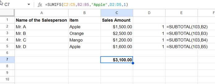
This range can be called the helper column range.
What do these formulas (helper column range) do?
The SUBTOTAL function with the code 103 returns the count of each cell. It returns 1 if the cell has a value, else 0. When you hide a row, the formula will return 0, irrespective of whether it has a value or not.
We will use this feature in the following SUMIFS formula:
=SUMIFS(C2:C5,B2:B5,"Apple",D2:D5,1)Syntax:
SUMIFS(sum_range, criteria_range1, criterion1, [criteria_range2, …], [criterion2, …])Where:
sum_rangeisC2:C5criteria_range1isB2:B5criterion1is"Apple"criteria_range2isD2:D5criterion2is1
This SUMIFS formula calculates the total of “Apple” in visible rows.
The formula in cell C7 is a SUMIFS formula that does the subtotal with the condition in Google Sheets.
Instead of SUMIF, I have used the SUMIFS function because we want to check two conditions:
- The value in column B is “Apple.”
- The value in column D is greater than 0.
Column D is our new column with a few SUBTOTAL formulas. When you hide any rows or apply a filter, the hidden row value in column D will become zero. So, the SUMIFS formula excludes such rows in the sum.
SUBTOTAL with Conditions Without Using a Helper Column in Google Sheets
I know most of you are not in favor of using a helper column range. Me too.
We can do subtotal with conditions without using any helper column range in Google Sheets. What you want to do is to use the SUBTOTAL function with MAP.
We can expand the D1 formula on its own with the help of the MAP function.
=MAP(B2:B5, LAMBDA(row, SUBTOTAL(103,row)))Replace criteria_range2 in the formula, i.e., D2:D5 with this formula. It will be as follows.
=SUMIFS(C2:C5,B2:B5,"Apple",MAP(B2:B5, LAMBDA(row, SUBTOTAL(103,row))),1)Conclusion
We have seen how to use SUBTOTAL with conditions in Google Sheets. If you want to explore the possibilities of SUBTOTAL with conditions further, there are a few more tutorials available. Here they are:
- How to Omit Hidden or Filtered Out Values in Sum
- SUMIF Excluding Hidden Rows in Google Sheets
- Google Sheets Query Hidden Row Handling with Virtual Helper Column
- Vlookup Skips Hidden Rows in Google Sheets
- Insert Sequential Numbers Skipping Hidden | Filtered Rows in Google Sheets
- COUNTIF | COUNTIFS Excluding Hidden Rows in Google Sheets
Hi,
1.Subtotal Works if Rows are Hidden for a column
2.but does not work if columns are hidden for a Row.
How can we use this when we need to sum Rows? [ Cannot transpose as I also Have Sparklines etc.]
Hi, Apurva,
As far as I know, there is no built-in function in Google Sheets that we can use to identify hidden columns.
You may sometimes find Apps Script. Search “StackOverflow”.