There are two random number generator functions in Google Sheets. They are RAND and RANDBETEEEN volatile Google Sheet functions. This time we can learn how to use RAND and RANDBETWEEN functions in Google Sheets.

There is not much complication in using RAND and RANDBETWEEN functions. They are just random number generators. You can very easily understand it and start to begin using it.

Update: There is one more new similar function called RANDARRAY. Read about that here – How to Use the RANDARRAY Function in Google Sheets.

Use of RAND and RANDBETWEEN Functions in Google Sheets

Let us start with the RAND Google Spreadsheet function.

RAND Function in Google Sheets

You can directly use RAND function in any cell to generate a random number as, unlike RANDBETWEEN, it doesn’t take any arguments.

Here is the syntax.

=RAND()

This function returns a random number between 0 inclusive and 1 exclusive. That means the Google Sheets RAND formula can return a random number between 0 and 0.9999999.

Suppose in cell A1, you’ve inserted the above RAND function. Then you will get one random number. If you delete and again insert the RAND formula, this time you will get a new random number.

The reason RAND is a volatile function and that’s why this function called random number generator.

The random number thus generated will be subject to change similar to the TIME as well as DATE Google Sheets functions.

I mean, when you make any changes to your spreadsheet, the random number will get change similar to the NOW() function. But you can control the frequency of this change like every minute, every hour, etc. That setting you can find here.

Example to the RAND Google Sheets Function

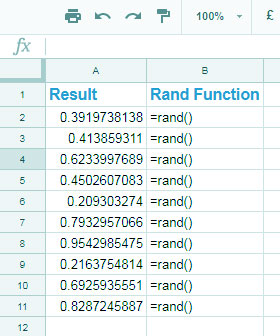
The main purpose of Google Sheets RAND function is to generate a random number between 0 and 1.

Just check the below screenshot. Nothing more to explain about RAND function at this point.

RANDBETWEEN Function in Google Sheets

Unlike RAND Google Sheets function, RANDBETWEEN function takes arguments in it. Below is the syntax.

Syntax

RANDBETWEEN(low, high)

Arguments

low – The low end (the smallest integer) of the random range.

high – The high end (the largest integer) of the random range.

Here you can define high and low values. This formula can return a random integer between two values, both inclusive.

Example to the RANDBETWEEN Google Sheets Function

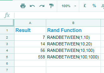
In the below examples, formula one returns a random number between 1 and 10 both inclusive.

The second formula returns a random number between 10 and 20. The other formulas in the example follow this pattern.

How to Use RAND Function Instead of RANDBETWEEN Function (The Flexible Random Number Generator)

For me, the RAND function is more flexible. We can use it instead of RANDBETWEEN in combination with other functions.

You can easily get a unique integer between 0 to 100, where 100 is not inclusive, with the following RAND and TRUNC function combination.

=trunc(rand()*100)

Similarly 0 to 10, here also 10 is not inclusive.

=trunc(rand()*10)

You can further expand the usage of RAND function and to make it just to behave like RANDBETWEEN function.

In RAND function also you can apply low and high-value arguments indirectly. For this, we can use the same above TRUNC and RAND combination.

In the above, we can only have control over the largest value. We can overcome this by deducting our desired lower value from the output.

=trunc(rand()*(100-10)+10)

It will return a random number between 10 to 100. Here 100 is the largest and 10 is the lowest argument. Here 10 is inclusive but 100 not. See one more example (1 lowest, 9 largest).

=trunc(rand()*(10-1)+1)

Hope you have enjoyed these tips. See you again with a practical example to the RANDOM number in Google Sheets.

Related:

1. How to Pick a Random Name from a Long List in Google Sheets.
2. How to Shuffle Rows in Google Sheets Without Plugin.
3. Pick Random Values Based on Condition in Google Sheets.
4. How to Randomly Select N Numbers from a Column in Google Sheets.
5. How to Randomly Extract a Certain Percentage of the Rows in Google Sheets.
6. Google Sheets: Macro-Based Random Name Picker.
7. How to Generate Odd or Even Random Numbers in Google Sheets.