


This post elaborates on the proper usage of text, numeric, and date criteria in the DSUM function within Google Sheets.
In this tutorial, I won’t delve into the basic usage of the DSUM function as it’s already covered here: How to Use the DSUM Function in Google Sheets. Additionally, you can explore various comprehensive DSUM tutorials by utilizing the search option on this site or referring to the “Resources” section provided at the end.
Here my topic is different. Here I will tell you how to properly use criteria in DSUM, whether it should be within double quotes (text), without double quotes (numeric), or in any other specific format (date and time).
When considering the proper use of criteria, there are certainly two main aspects to consider. What are they?
The first aspect involves using criteria within the formula itself (hard-coded), while the second aspect entails using criteria as a cell reference. I’ll cover both of these approaches.
Let’s now delve into how to properly use text, numeric, and date criteria within the DSUM function.
Google Sheets: How to Properly Use Criteria in DSUM
I’ve prepared a reference table for you to consult whenever you encounter difficulties using criteria in DSUM.
Syntax: DSUM(database, field, criteria)Focus on the ‘criteria’ part of the syntax. I’ll guide you through the proper use of text, numeric, and date criteria here. Refer to the chart below for details.
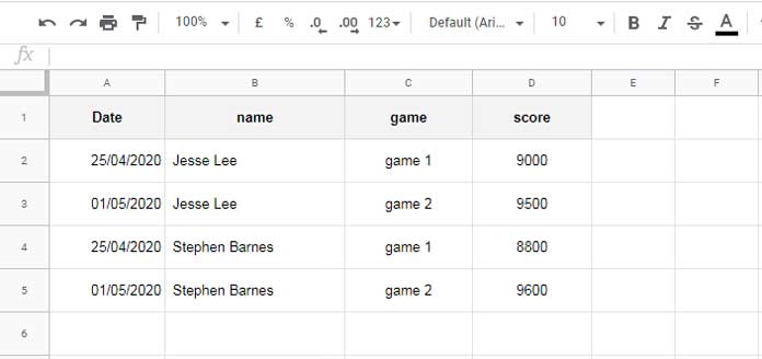
Sample Data with Field Labels (Header Row)
The sample data should contain field labels, resembling a database table, with no merged cells present. Here is a sample dataset for use in examples. The data range is A1:D, where cell range A1:D1 contains the field labels (header row).
DSUM Criteria Reference Chart (Table) Based on Sample Data
| Type | Within Formula (Hardcoded) | When Using F1:F2 (Criteria Reference) |
| Text | VSTACK("name", "Jesse Lee") | F1: name F2: Jesse Lee |
| Numeric | VSTACK("score", 9600) | F1: score F2: 9600 |
| Numeric with Operators | ||
| > | VSTACK("score", ">"&9000) | F1: score F2: >9000 |
| < | VSTACK("score", "<"&9000) | F1: score F2: <9000 |
| <> | VSTACK("score", "<>"&9000) | F1: score F2: <>9000 |
| >= | VSTACK( "score", ">="&9000) | F1: score F2: >=9000 |
| <= | VSTACK("score", "<="&9000) | F1: score F2: <=9000 |
| Date | VSTACK("date", DATE(2020, 4, 25))Date as per the syntax DATE(year, month, day) | F1: date F2: 25/04/2020 DD/MM/YYYY or MM/DD/YYYY (as per your settings) |
| Date with Operators | ||
| > | VSTACK("date", ">"&DATE(2020, 4, 25)) | F1: date F2: =">"&DATE(2020, 4, 25) |
| < | VSTACK("date", "<"&DATE(2020, 4, 30)) | F1: date F2: ="<"&DATE(2020, 4, 30) |
| <> | VSTACK("date", "<>"&DATE(2020, 5, 1)) | F1: date F2: ="<>"&DATE(2020, 5, 1) |
| >= | VSTACK("date", ">="&DATE(2020, 4, 25)) | F1: date F2: =">="&DATE(2020, 4, 25 |
| <= | VSTACK("date", "<="&DATE(2020, 4, 30)) | F1: date F2: ="<="&DATE(2020, 4, 30) |
In the DSUM criteria usage chart above, the column names (field labels) correspond to the following meanings.
Legends
- Type: Indicates the type of criteria – text, numeric, or date.
- Within formula: Refers to the criteria format when hardcoded into the formula.
The VSTACK function is utilized to vertically stack the fields labeled with the criterion. Also, please note that the DATE function in the criterion follows the syntax DATE(year, month, day).
Previously, we were using curly brackets to create the criteria array in DSUM or other database functions in Google Sheets. For example, instead of VSTACK("name", "Jesse Lee"), you can use {"name"; "Jesse Lee"}.
When you need to refer to a 2D array as criteria and hardcode it, you may need to use a combination of VSTACK and HSTACK functions.
| name | game |
| Jesse Lee | game 1 |
If the table on the left represents the criteria, you can code it as VSTACK(HSTACK("name", "game"), HSTACK("Jesse Lee", "game 1")).
Here are a few examples to help you understand how to utilize the DSUM criteria usage chart provided above.
Text Criteria
- Proper use of Text Criteria in DSUM within the formula:
=DSUM(A1:D5, 4, VSTACK("name", "Jesse Lee")) - Proper use of Text Criteria in DSUM as a cell reference:
=DSUM(A1:D5, 4, F1:F2)
Date Criteria
- Proper use of Date Criteria in DSUM within the formula:
=DSUM(A1:D5, 4, VSTACK("date", DATE(2020, 4, 25))) - Proper use of Date Criteria in DSUM as a cell reference:
Please follow the formula provided under point #2 above.
Numeric Value as Criteria
- Proper use of Numbers as Criteria in DSUM within the formula:
=DSUM(A1:D5, 4, VSTACK("score", 9600)) - Proper use of Numbers as Criteria in DSUM as a cell reference:
Please follow the formula provided under point #2 above.
You can also observe the comparison operators used with criteria in DSUM.
If you found this tutorial helpful, feel free to bookmark this page for future reference.
Resources
- How to Use Date Difference as Criteria in DSUM in Google Sheets
- Difference Between SUMIFS and DSUM in Google Sheets
- Comparing SUMIFS, SUMPRODUCT, and DSUM with Examples in Google Sheets
- How to Do a Case-Sensitive DSUM in Google Sheets
- AND, OR in Multiple Criteria DSUM in Google Sheets (Within Formula)
- Google Sheets: How to Use Multiple Sum Columns in DSUM Function