


")


The purpose of the MATCH function in Google Sheets is to return the relative position of an item in a list (relative position refers to the position of an item within a list or range).
Tip: However, the function can be used to find the row number when searching vertically and the column number when searching horizontally.
Real-life Use: We can use the output of the MATCH function with functions like INDEX or FILTER to get specific values from that range or outside the range.
Let’s explore this with the examples below. As a side note, Google Sheets introduced a newer function called XMATCH, which provides additional features.
Syntax and Arguments
Please go through the syntax section carefully as I’ve included some important tips in between.
Syntax:
MATCH(search_key, range, [search_type])Arguments:
search_key:The value (text, number, or date) to search for.range: The one-dimensional array to be searched. If thesearch_keyis “Apple” and therangeis A2:A10, the formula will return the position of “Apple” in this range. To get the row number, specify A:A instead. This applies to horizontal ranges as well.search_type: This is an optional argument with a default value of 1.- 1: Use when your range is sorted in ascending order (matches the largest value less than or equal to the
search_key). - -1: Use when your range is sorted in descending order (matches the smallest value greater than or equal to the
search_key). - 0: Use when the range is not sorted (exact match).
- 1: Use when your range is sorted in ascending order (matches the largest value less than or equal to the
When the range is not sorted, if you omit or incorrectly specify 1 or -1 as the search_type in your MATCH formula, the formula may return an incorrect result. This is one of the most common errors that users encounter when using the MATCH function in Google Sheets.
MATCH Function in an Unsorted Range in Google Sheets
We will begin by using the MATCH function in an unsorted range, which is the most common use case for this function. In this scenario, you need to specify the search_type as 0.
Text String as Search Key
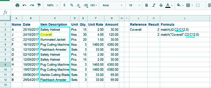
In the following example, I aim to search for the value “Coverall” in the range C2:C12 using the MATCH function to determine its relative position within this range.
=MATCH("Coverall", C2:C12, 0) // search key is hardcoded in the formula
=MATCH(J2, C2:C12, 0) // search key is in cell J2
The above formula will return 2 since it matches the value “Coverall” in cell C3. Please refer to the image below.
Notes:
- If there are multiple occurrences of the search key in the range, the formula will return the position of the first occurrence.
- To find the row number, specify C:C as the range.
- If there is no match, the formula will return the #N/A error. To handle this, you can wrap your formula with the IFNA function like so:
=IFNA(MATCH(J2, C2:C12, 0)).
Numeric Value as Search Key
The following formulas search for the number 1460 in the range F2:F12 and return its position:
=MATCH(1460, F2:F12, 0) // search key is hardcoded in the formula
=MATCH(J6, F2:F12, 0) // search key is in cell J6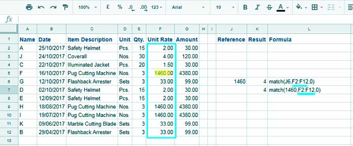
Date as Search Key
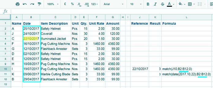
When utilizing a date as the search key in the MATCH function, there are some considerations. If the search key is a cell reference, there’s no issue:
=MATCH(J10, B2:B12, 0) // search key in cell J10However, if the search key is hardcoded within MATCH, then it’s advisable to use the DATE function to properly specify the criterion (search_key):
=MATCH(DATE(2017, 10, 22), B2:B12, 0) // search key is hardcoded in the formulaSyntax: DATE(year, month, day)
MATCH Function in a Sorted Range in Google Sheets
Let’s consider the range A1:A5 containing the numbers 1, 5, 6, 10, and 15 respectively, sorted in ascending order.
The following MATCH formula will return 3 since the search key 8 is not in the range, and the relative position of the largest value less than the search key is 6, with its position being 3:
=MATCH(8, A1:A5, 1)Now, assuming the same numbers in descending order, like 15, 10, 6, 5, 1, and using the search key 8 with search_type -1, the MATCH will return 2.
It’s because the smallest value greater than or equal to the search key is 10, and its relative position is 2:
=MATCH(8, A1:A5, -1)If the search key is available, there is no issue. It will return the position of the exact match in both ascending and descending sorted ranges.
MATCH Function with FILTER Function in Google Sheets
The MATCH function in Google Sheets can indeed match multiple search keys. When doing so, you should use ARRAYFORMULA with it.
In the following example, I have a few employee names in column A and their salary advances in column B. The range is A1:B7.
We will use the names in A1:A7 as the search keys in a MATCH formula, and the range F1:F2 contains two employee names.
The following MATCH formula will return an array result with relative positions for matches and #N/A for mismatches:
=ArrayFormula(MATCH(A1:A7, F1:F2, 0))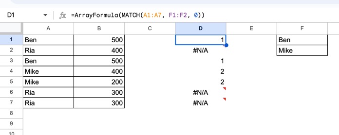
We can use this array result as a condition in a FILTER formula to return the salary advances of the persons specified in F1:F2. The ARRAYFORMULA is not required within FILTER:
=FILTER(B1:B7, MATCH(A1:A7, F1:F2, 0))Syntax: FILTER(range, condition1, [condition2, …])
Using the MATCH Function Inside the INDEX Function
To understand this usage, you must first know the syntax of the INDEX function, which is as follows:
INDEX(reference, [row], [column])In the following table, range A1:B6, we can use the MATCH function to match “Grape” in A1:A6 and use INDEX to get the corresponding price from B1:B6:
| Apple | 5 |
| Orange | 4.5 |
| Mango | 5.25 |
| Banana | 3.25 |
| Pineapple | 4.75 |
| Grape | 6 |
=INDEX(B1:B6, MATCH("Grape", A1:A6, 0))This is an example of dynamic row offset in INDEX using the MATCH function in Google Sheets.
Related: Index Match: Better Alternative to Vlookup and Hlookup in Google Sheets
Conclusion
In all the above examples, we have used MATCH in a vertical array. Similarly, you can use it in a horizontal array without changing the arguments used.
For example, if the range is C1:Q1, the formula will return the relative position of the search key. If you want the column number instead, use 1:1 as the range.
Another aspect is using the MATCH function inside the INDEX function. In such cases, when the range is a horizontal array, use the MATCH formula in the column argument of the INDEX function.
Hi Prashanth 🙂
I would like to ask you regarding MATCH function.
If I have 2 tables with the same name and column such as :-
TABLE A : [Name, Age, Address] TABLE B : [Name, Age, Address]
I want to make another table (TABLE C-with the same column & name) , to combine both data in the new table. But, if the row in TABLE A is match with TABLE B, it will take only one row instead of taking both rows (if it takes both, the data is redundant).
Is it possible to use MATCH or any other formula for it?
Thank you so much 🙂
https://infoinspired.com/google-docs/spreadsheet/merge-two-tables-in-google-sheets/