


We can use various options to limit the number of rows in the processed data in the Google Sheets QUERY function.
There are two QUERY language clauses – OFFSET and LIMIT. Additionally, we can encapsulate the formula with either ARRAY_CONSTRAIN or the CHOOSEROWS function.
The LIMIT clause, ARRAY_CONSTRAIN, and CHOOSEROWS functions are used to limit the number of rows in the aggregated data. The OFFSET function, on the other hand, is employed to offset a certain number of rows from the beginning of the processed data.
Sample Data
The sample data comprises items, salesperson, quantity, and amount in the range A1:D.
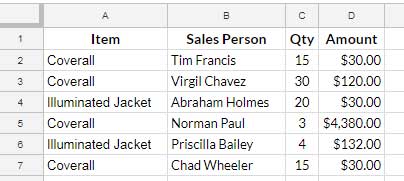
There are multiple occurrences of two items. We will group the items, sum the amounts, and sort the results.
Let’s limit the number of rows to 1 using QUERY or two other functions.
LIMIT Clause to Limit the Number of Rows in QUERY
We will explore the use of the LIMIT clause to restrict the number of rows in two steps. Let’s begin with understanding the syntax.
Syntax of the QUERY function: QUERY(data, query, [headers])
Step 1 Formula:
=QUERY(A1:D, "SELECT A, SUM(D) WHERE A IS NOT NULL GROUP BY A LIMIT 1", 1)Result:
| Item | sum Amount |
| Coverall | 4560 |
Where:
- data: A1:D
- query:
"SELECT A, SUM(D) WHERE A IS NOT NULL GROUP BY A LIMIT 1"SELECT A, SUM(D): Select column A and calculate the sum of values in column D.WHERE A IS NOT NULL: Filters out any rows where column A is empty.GROUP BY A: Groups the results by values in column A.LIMIT 1: Limits the result to just one row.
- headers: 1 (The data has a header row.)
Step 2: Sorting the aggregated values and limiting the rows:
When you don’t specify the ORDER BY clause, the output of the query formula will be sorted by the columns in the GROUP BY clause.
To limit the number of rows after sorting, use the ORDER BY clause. Here is an example:
=QUERY(A1:D, "SELECT A, SUM(D) WHERE A IS NOT NULL GROUP BY A ORDER BY SUM(D) ASC LIMIT 1", 1)Result:
| Item | sum Amount |
| Illuminated Jacket | 162 |
This formula will sort the grouped results based on the sum of values in column D in ascending order.
If you’re unfamiliar with QUERY language clauses, please refer to this guide: What is the Correct Clause Order in Google Sheets Query?
Offsetting Rows in Google Sheets QUERY
Offsetting rows is another way of limiting the number of rows in Google Sheets QUERY.
In some scenarios, you might need to skip a certain number of rows from the beginning of the QUERY results. This is where the OFFSET clause in QUERY becomes relevant.
In the following formula, we use the LIMIT clause to restrict the rows to 2 and OFFSET to skip 1 row. So even though the number of rows limited is 2, the output will contain only 1 row due to the offset.
=QUERY(A1:D, "SELECT A, SUM(D) WHERE A IS NOT NULL GROUP BY A ORDER BY SUM(D) ASC LIMIT 2 OFFSET 1", 1)Limiting Number of Rows in QUERY Using CHOOSEROWS or ARRAY_CONSTRAIN
You can restrict the number of rows without using the LIMIT clause in QUERY.
Here’s how to utilize ARRAY_CONSTRAIN as well as CHOOSEROWS with QUERY for this purpose:
Base QUERY Formula:
=QUERY(A1:D, "SELECT A, SUM(D) WHERE A IS NOT NULL GROUP BY A", 1)Using ARRAY_CONSTRAIN:
Syntax: ARRAY_CONSTRAIN(input_range, num_rows, num_cols)
Formula:
=ARRAY_CONSTRAIN(QUERY(A1:D, "SELECT A, SUM(D) WHERE A IS NOT NULL GROUP BY A", 1), 2, 2)Where:
input_rangeis the QUERY formula,num_rowsis 2 (including the header row), andnum_colsis 2.
Using CHOOSEROWS:
Syntax: CHOOSEROWS(array, [row_num1, …])
Formula:
=CHOOSEROWS(QUERY(A1:D, "SELECT A, SUM(D) WHERE A IS NOT NULL GROUP BY A", 1), SEQUENCE(2))Where:
arrayis the QUERY formula, androw_num1is SEQUENCE(2). Within SEQUENCE, specify the number of rows to limit including the header row.
This approach has a slight advantage over others. You can use SEQUENCE to dynamically control the extraction of rows:
For example, if you want to extract the last 5 rows, use the following SEQUENCE:
=SEQUENCE(5, 1, -1, -1)(Our sample data is very small and doesn’t contain 5 rows. So you can test it with a larger dataset.)
Resources
Here are some interesting tutorials to read about QUERY.
- How to Use And, Or, and Not in Google Sheets Query
- How to Use Cell Reference in Google Sheets Query
- CONTAINS Substring Match in Google Sheets Query for Partial Match
- Multiple CONTAINS in WHERE Clause in Google Sheets Query
- How to Use Date Criteria in Query Function in Google Sheets [Date in Where Clause]
Hi Prashanth,
I’m trying to skip the lines that contain years, as I only want to list the months.
Any idea how to achieve this?
Many thanks,
René
Hi, René,
To filter G37:K to a new range only for the rows that contain month texts in G37:K, you can try the below FILTER.
=filter(G37:K,regexmatch(G37:G&"","[0-9]")=FALSE)Hi Prashanth,
I am trying to get the top 15% by sector, but when I use function
=QUERY(ARRAY_CONSTRAIN(SORT($A$7:$S,10,FALSE),15,23), "Select Col1, Col8, Col3, Col10"), it displays the data incorrectly.Could you please advise me what I am doing wrong?
Hi, Ron,
The above formula works like this.
1. Sorts column 10 (Change %) in descending order – SORT.
2. Constrains the number of rows to 15 – ARRAY_CONSTRAIN.
3. Limit the number of columns to 4 – Query.
All that you can do with the below Query itself!
=QUERY({'Sector Perf'!$A$7:$BR},"Select Col1, Col8, Col9, Col10 order by Col10 desc limit 15")But that doesn’t address your problem. Can you explain what you want to achieve?
If I want to take only the last row, what function is properly?
Hi, Alex Daniel,
To filter the last row in the range A2:D.
=array_constrain(SORT(A2:D,ROW(A2:A)*N(A2:A<>""),0),1,4)I’ve flipped the data then using Array_Constrain, limited the output number of rows to 1.