In Google Sheets, the IMPORTRANGE formula can connect two sheets and import data between them. The Query is another awesome function in Google Sheets. By using Query with IMPORTRANGE you can apply conditional import range. Here is an example of conditional Importrange in Google Sheets. Below is the step by step tutorial on how to Import a Range with Less Than or Greater Than in Google Sheets with the help of Query.
We can use the Less than or Greater than comparison operators to date as well as numeric fields in Importrange with the help of other functions and mainly Query. We are going to learn this technique here. You may want to refer the below tutorials.
1. Learn Query Function in Google Sheets.
2. Google Sheets IMPORTRANGE function.
Import a Range With Less Than or Greater Than in Google Sheets
First I am going to explain to you how to apply less than “<” or greater than “>” comparison operators in a column containing dates.
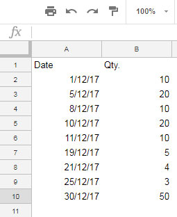
Sample Data in Google Sheet 1:

From this sample data, let me answer the following.
How to Import a Range from Another Google Sheets Between Dates
In Google Sheet 2 you can use the below Importrange formula to import the entire data as it is.
=importrange("URL","Sheet1!A1:B10")
Here you just need to replace URL with the original URL of Google Sheet 1. Now with a Query formula that wrapping the Importrange, we can apply conditional Importrange in Google Sheets.
It’s time to scroll back to the top and check the sample data in Column 1. You can see that Column 1 contains certain dates.
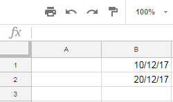
Here in Google Sheet 2, I’m importing Column 1 from Google Sheet 1 where the date falls between 10/12/2017 and 20/12/2017, both the dates inclusive.

I have the criteria in Cell B1 and B2 in Google Sheet 2. So here is the formula in Google Sheet 2 to import the data from Google Sheet 1.
Formula 1:
=query(importrange("URL","Sheet1!A1:B"),"Select * where Col1>=date' "&TEXT(B1,"yyyy-mm-dd")&" ' and Col1<=date' "&TEXT(B2,"yyyy-mm-dd")&" ' ",1)
Explanation:
When you Import a Range With Less Than or Greater Than in Google Sheets, you should know how to use less than “<” or greater than “>” comparison operators in Query.
The Date criteria in Cell B1 and B2 is in “dd/mm/yy” format. But with Query, we can only use the “yyyy-mm-dd” format.
In your leisure, you may please follow my below two tutorials for detailed information in this regard.
How to Use Date Criteria in Query Function in Google Sheets
Convert Date to String Using the Long-winded Approach in Google Sheets
How to Import a Range from Another Google Sheets Between Numeric Values
Here also the formula pattern follows the formula 1 above. But this time the “Where” clause in Query will be as follows. Here the criteria are in C1 and C2.
where Col1>="&C1&" and Col1<="&C2&"
How to Sum or Count Data in Another Google Sheets Between Certain Dates
Here I am using the above sample data and formula 1. We only need to make changes to the formula as below.
Formula 2:
=sum(query(importrange("URL","Sheet1!A1:B"),"Select Col2 where Col1>=date'"&TEXT(B1,"yyyy-mm-dd")&"' and Col1<=date'"&TEXT(B2,"yyyy-mm-dd")&"'",1))
The difference with Formula 1:
Here I’ve just wrapped the formula 1 with the SUM function. Additionally, in formula 1, it’s Select “*”, here instead, I’ve only imported the column that we want to SUM that is Col2.
Instead of SUM, you can use COUNT to count an imported data between dates or numeric values.
That’s all for now. Like to hear your views in comments.


Hi Prashanth,
Thank you very much for the tutorials and for your effort.
Can I share with you my sheets, of course without personal data? Could you please help me? I have to import data for the blue criteria (Sheet Test 02, Report): Column C 7,8 & 10,11. I can offer payment for your effort, it is very important for me.
— Links removed by Admin —
Thank you in advance!
Anita
Hi,
Sent request for access to your Sheets. I’ll try to help you!
Hi, Anita,
Please correct the date entered in cell G2,G3, and G47 (Sheet: Copy of Test 1, Tab: Professional Test). The date format is wrong. There are other issues.
I am not going into the detail of the solution here as other readers may not find it useful. So I am sending back you the files (I have made copies of the files for editing) via email.
Best,
Dear Prashanth,
First of all, thank you very much for this website, you are doing a great job.
I have the following problem, could you please help me?
I have 2 separate Spreadsheets, one of them contains a column with “Received date (for the whole year)”, the second one contains columns for each calendar week separately.
I have to import data from the first file to the other one, and I need a function that counts how many requests I received for each week separately.
For example, how many requests have I received in week 6 (04/02/2019-10/02/2019)?
Please 🙂
Anita
Hi, Anita,
I’ll try to help you with an example soon. Once I am ready with that tutorial, I’ll update you.
Best,
See if this tutorial helps?
How to Count Orders Per Week in Google Sheets
Just a little correction: Formula1 doesn’t work as typed. There are extra spaces within the single quotes enclosing the date to text conversions that throws a parsing error.
Instead of:
"&TEXT(B1,"yyyy-mm-dd")&" ' and Col1<=date' "&TEXT(B2,"yyyy-mm-dd")&" ' ",1)it should be:
"&TEXT(B1,"yyyy-mm-dd")&"' and Col1<=date' "&TEXT(B2,"yyyy-mm-dd")&"' ",1)Otherwise an excellent set of tutorials. Thank you very much! They've helped me considerably.
Sorry that 2nd line should be:
“&TEXT(B1,”yyyy-mm-dd”)&”‘ and Col1<=date'"&TEXT(B2,"yyyy-mm-dd")&"'",1)
Another space somehow made it into the formatting. HTML formatting problem on the site instead?
Hi, Ken,
You are right! I myself noticed that in the past.
I am posting the formulas after a thorough test from my side. But the issues happen when I publish my posts. If I post the formulas as CODE then the spacing issue happens and may often affect the Query formulas.
If I post the formulas as plain text formats, then the double/single quotes may cause the issue.
So the solution is to remove the extra space between single Double quotes in Query formulas (if the formula is posted as CODE) else retype the single double quotes.
Thanks for the time taken to notify me.