


Don’t limit your Vlookup experiment to a single search key and single-cell result. You can do a lot more with Vlookup. Here we can learn the tips to use Vlookup to return an array result in Google Sheets. I hope you don’t confuse with my earlier two advanced Vlookup tutorials handling a similar topic. What are they?
1. How to Return Multiple Values Using Vlookup in Google Sheets? – Here the Vlookup formula uses a single search key to find a match in the first column and returns multiple values from the same row of the match found.
2. How to Use VLOOKUP with Multiple Criteria in Google Sheets? – In this case, we are making use of a helper column to combine values in two columns and use this column as our Vlookup first column to lookup. So the Vlookup search key would also be a combined key.
But in this tutorial, I am using an entire column as search key column with the help of ARRAYFORMULA and find all matches in the first column of another data set and return the result as an array. You can easily grasp this point from the example below.
Similar: Case Sensitive Vlookup in Google Sheets
Tips to Use Vlookup to Return An Array Result in Google Sheets
As I have mentioned, you can use the function Vlookup to return an array result as below in Google Doc Spreadsheets.
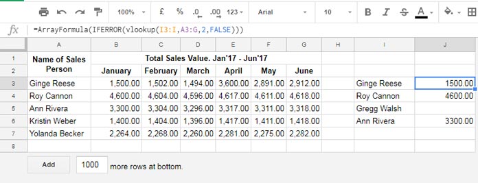
In Column I3:I, you can see a few names of Sales Persons. The Vlookup formula in the cell J3 searches down these names in the first column of the range A3:G and then returns the result from the second column.
If there is no match, the formula would return blank cell as output. That’s why cell J5 is blank. There is no name with “Gregg Walsh” in the first column of the lookup range.
Of course, I will explain to you how this Vlookup Array Formula is different from the normal one, which you may be familiar with.
Formula 1:
Vlookup to Return An Array Result in Google Sheets
=ArrayFormula(IFERROR(vlookup(I3:I,A3:G,2,FALSE)))The above formula is equal to;
=ArrayFormula(IFERROR(vlookup({"Ginge Reese";"Roy Cannon";"Gregg Walsh";"Ann Rivera"},A3:G,2,FALSE)))Formula 2:
Basic Vlookup Formula.
=vlookup(I3,A3:G,2,FALSE)And the above formula 2 is equal to;
=vlookup("Ginge Reese",A3:G,2,FALSE)Just compare the formula 1 with the formula 2 and understand the difference.
In Formula 1 I’ve used a column I3:I as the search key column in Vlookup. But in Formula 2 it is just the cell reference I3.
Here the first Vlookup formula uses an array as Search Key and returns an array result. So that we should wrap the Vlookup formula with the ArrayFormula.
I hope you may know the use of IFERROR already. The role of it’s to remove #N/A! or any other errors returned by Vlookup.
If you are just concerned with #N/A! errors, better to use IFNA which is relatively a new function.
This way, you can use Vlookup to return an array result in Google Sheets.
Conclusion
By learning advanced tips of using functions like Vlookup, Sumproduct, Sumif, and Query you can save lots of man-hours.
For example, the above single Vlookup formula could replace multiple Vlookup formulas.
So learn the advanced use of Google Sheets functions and improve your efficiency in your job.