Understanding time functions are very important when you have to handle salary, payroll, etc. Similar to the date-related functions, time is also an important factor in such calculations. So let me explain how to use all different time formulas in Google Sheets.

If you are not yet familiar with date functions in Google Sheets, switch to our date formulas guide – Learn All Google Sheets Date Formulas.

Master the below all different time formulas in Google Sheets so that you can face any time-related calculations with ease.

When we talk about all different time formulas, there are seven functions in Google Sheets related to time. All are easy to use and understand.

Example to Time Formulas in Google Sheets

TIME Function in Google Sheets

How to use the Time function in Google Sheets?

The purpose of the Time function in Google Sheets is to return provided hour, minute and second into time.

TIME Function Syntax:

TIME(hour, minute, second)

Formula example to the use of the TIME function in Docs Sheets.

You can enter hours, minutes and seconds components in different cells and combine them as a time using the TIME function in Sheets.

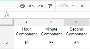
=TIME(A2,B2,C2)

Another example of the above Time formula is;

=TIME(10,35,59)

NOW Function in Google Sheets

How to use the Now function in Google Sheets?

The purpose of the NOW function in Google Sheets is to return the current date and time. It’s a volatile function.

Volatile function – What does it mean in Google Sheets?

A volatile function updates automatically in the cell where it resides. It updates every time when a user edits the Spreadsheet.

NOW Function Syntax:

NOW()

In the cell C5 or in any blank cell, enter this formula.

=NOW()

The above NOW formula in Google Sheets will return the current time in the timestamp format.

03/10/2017 10:18:49

Here you may normally raise the following two questions.

1. How to get the current time without the date in Google Sheets?
2. How to remove the date from the date time or NOW formula output?

The answers to both the above questions are the same. There are two options in Docs Sheets to extract the current time from the time and date format.

Option # 1:

Using a time formula and the Format menu.

First, apply the below formula in any cell to get the current time value.

=NOW()-TODAY()

Keep that cell active. Then go to the menu Format > Number and select the “Time” format.

Option # 2:

Using the Text function with NOW() you can get the current time without the date in Google Sheets.

=TEXT(NOW(),"hh:mm:ss")

HOUR Function in Google Spreadsheets

How to use the Hour function in Google Sheets?

The purpose of the HOUR function in Google Sheets is to return the hour component from the given time.

HOUR Function Syntax:

HOUR(time)

See the below two example formulas. I hope that can help you to understand how to use the HOUR function in Sheets.

Formula 1:

=HOUR("11:40:59")

Formula 2:

=HOUR(TIME(A2,B2,C2))

Here please refer to the TIME function example above.

MINUTE Function in Google Docs Sheets

How to use the Minute function in Google Sheets?

This function is similar to the HOUR function. It returns the minute component of a given time. So I don’t want to repeat the examples here.

MINUTE Function Syntax:

MINUTE(time)

SECOND Function in Sheets

How to use the Second function in Google Sheets?

The SECOND function in Google Sheets is also similar to the HOUR and MINUTE functions above. It returns the seconds component of a given time. Just see the syntax.

SECOND Function Syntax:

SECOND(time)

TIMEVALUE Function in Google Sheets

How to use the Timevalue function in Google Sheets?

The TIMEVALUE function returns the time value, i.e. the fraction of a 24-hour day the time represents.

TIMEVALUE Function Syntax:

TIMEVALUE(time_string)

You can use this formula in either 24 hour or 12 hour format.

The TIMEVALUE formula example in 24 Hrs. Format:

=TIMEVALUE("11:10:15")

The TIMEVALUE formula example in 12 Hrs. Format:

=TIMEVALUE("11:10:15 AM")

The above formula result will be the value “0.4654513889”.

This value you can use for your different time-related operations. When you want to convert this numeric value back to time use the text formula as;

=text(E24,"hh:mm:ss")

Also you can use the Format menu to convert time values back to normal time.

Note: If you refer to a cell that contains time in the TIMEVALUE function, it would return #N/A error.

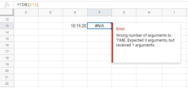
In such case, you can use the below To_pure_number function.

TO_PURE_NUMBER Function in Google Docs Sheets

How to use the To_pure_number function in Google Sheets?

This is actually a Parser function and you may be new to this. Learn how to use the TO_PURE_NUMBER function in Google Sheets below.

TO_PURE_NUMBER Function Syntax:

TO_PURE_NUMBER(value)

This function converts and returns a pure number without formatting from a provided date/time, percentage, currency or other formatted numeric value. Didn’t get? See the below example.

Suppose in cell D2 there is time entered as 11:10:15. When you use the below formula you will get the time value of that time.

=TO_PURE_NUMBER(D2)

The result will be “0.4654513889”. This is similar to the TIMEVALUE function above. The difference is in TIMEVALUE we use string element in the formula, here time reference.

Formula:

=TO_PURE_NUMBER(25%)

Output: 0.25

Also, TO_PURE_NUMBER formula is not limited to time. This is similar to applying Format > Number > Automatic formatting option.

Related Time Formula Examples:

1. Convert Time Duration to Day, Hour, Minute in Google Sheets.
2. How to Deduct Lunch Break Time From Total Hours in Google Sheets.
3. How to Format Date, Time, and Number in Google Sheets Query.
4. Payroll Hours Time Calculation in Google Sheets Using Time Functions.
5. Google Sheets: The Best Overtime Calculation Formula.
6. How to Convert Military Time in Google Sheets.
7. Elapsed Days and Time Between Two Dates in Google Sheets.
8. Create a Countdown Timer Using Built-in Functions in Google Sheets.
9. How to Add Hours, Minutes, Seconds to Time in Google Sheets.
10. How to Format Time to Millisecond Format in Google Sheets.