Use the SUMPRODUCT function when you want to obtain the sum of products without first calculating the individual products and then summing them up. This approach is both a time and space saver.

You can specify two or more equal-sized arrays within this function, creating new possibilities. For instance, you can employ this function for conditional summing or product calculations. How?

You can use logical tests in a column to produce TRUE or FALSE (1 or 0). If a logical test returns 0, the product or the resulting value in that specific row will be 0.

Therefore, you can apply the SUMPRODUCT function in Google Sheets in scenarios similar to those where you would use SUMIF or SUMIFS.

Syntax and Arguments

Syntax:

SUMPRODUCT(array1, [array2, ...])

Arguments:

• array1: The first array whose values will be multiplied with corresponding values in the second array.
• array2: The second array whose values will be multiplied with corresponding values in the first array.

The second argument is optional. Therefore, if you only specify array1, the formula will simply return the sum.

Before diving into examples, you can make a copy of my sample sheet, which contains all the sample datasets and formulas we will detail in this tutorial.

Sample Sheet

SUMPRODUCT Example (Basic Use): Utilizing Two Arrays

Consider a scenario with two columns: quantities (array1) and prices (array2). To calculate the total cost, you can use the SUMPRODUCT function:

The sample data is in cell range A1:C5, where column A contains product names, B contains quantity, and C contains price. A1:C1 is designated for the field labels (header).

To obtain the total cost, you can use the following SUMPRODUCT formula:

=SUMPRODUCT(B2:B5, C2:C5)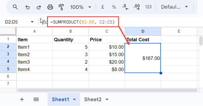

This is equivalent to:

=B2*C2 + B3*C3 + B4*C4 + B5*C5

LET Use Case:

=LET(
   quantity, B2:B5, 
   price, C2:C5, 
   SUMPRODUCT(quantity, price)
)

The LET use case proves beneficial when handling complex SUMPRODUCT formulas in Google Sheets. In this example, we utilized this function to assign meaningful names to the value expressions B2:B5 (named “quantity”) and C2:C5 (named “price”). These meaningful names were then used in the subsequent calculation, enhancing the clarity and readability of the formula.

SUMPRODUCT Example (Basic Use): Utilizing Three Arrays

Let’s consider a new scenario where we have a product column, quantity column, price column, and a discount percentage column.

This time we have the data in A1:D5, where A1:D1 is dedicated to the field labels.

The goal is to calculate the total cost after accounting for the discounts using the SUMPRODUCT function in Google Sheets.

Formula:

=SUMPRODUCT(B2:B5, C2:C5, 1-(D2:D5))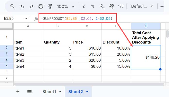

Which is equal to:

=(5 * 10 * (1-10%)) + (3 * 15 * (1-20%)) + (2 * 20 * (1-5%)) + (4 * 8 * (1-15%))

If you are wondering why deduct 1 from the discount percentage, i.e., 1 – D2:D5, it’s to create weightings that represent the complement of the discount percentages.

For example, if the discount is 10%, deducting it from 1 results in 90%, representing the portion of the original value retained after applying the discount.

LET Use Case:

=LET(
   quantity, B2:B5, 
   price, C2:C5, 
   discount, D2:D5, 
   SUMPRODUCT(quantity, price, 1-discount)
)

This LET function use case assigns meaningful names to the value expressions, enhancing the clarity and readability of the SUMPRODUCT formula.

Note: SUMPRODUCT is an array function in Google Sheets. Therefore, you do not need to explicitly specify the ArrayFormula function when using non-array value expressions, such as 1 – D2:D5, within this function.

Complex Use of the SUMPRODUCT Function in Google Sheets

Let’s revisit the above table with an added column, E2:E5, indicating “Yes” or “No.” If it’s “Yes,” the specified discount should be applied; otherwise, it shouldn’t.

Now, let’s address this complex scenario using the SUMPRODUCT function in Google Sheets:

=SUMPRODUCT(B2:B5, C2:C5, IF(E2:E5="Yes", (1 - D2:D5), 1))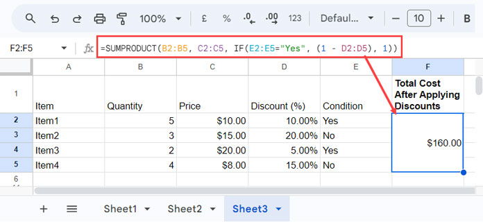

Where:

• array1: B2:B5
• array2: C2:C5
• array3: IF(E2:E5=”Yes”, (1 – D2:D5), 1)

Array3 introduces complexity to the SUMPRODUCT formula, incorporating an IF logical test. The formula assigns a weightage of 1 if the discount is not to be applied; otherwise, it uses (1 – D2:D5), representing the complement of the discount percentages.

LET Use Case:

=LET(
   quantity, B2:B5, 
   price, C2:C5, 
   discount, D2:D5, 
   condition, E2:E5, 
   SUMPRODUCT(quantity, price, IF(condition="Yes", 1-discount, 1))
)

SUMPRODUCT Function for Conditional Sum in Google Sheets

As mentioned earlier, specifying only array1 in the SUMPRODUCT formula sums the column range that the array represents. We’ve also explored a logical use case in the SUMPRODUCT example above.

Now, let’s leverage the SUMPRODUCT feature for multiple criteria conditional sums in Google Sheets.

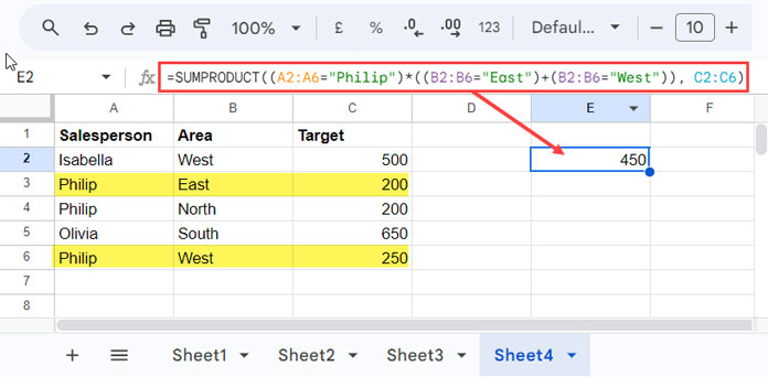
Consider the following table representing sales targets assigned to different salespersons:

Let’s see how to use SUMPRODUCT for conditional sums in its fullest diversity in Google Sheets.

We want to calculate the sales target of “Philip” from the areas “East” and “West.”

Formula:

=SUMPRODUCT((A2:A6="Philip")*((B2:B6="East")+(B2:B6="West")), C2:C6)

Where:

• array1: (A2:A6="Philip")*((B2:B6="East")+(B2:B6="West")).
  • This has two parts:
    • Part 1: (A2:A6="Philip") returns TRUE wherever the name matches.
    • Part 2: (B2:B6="East")+(B2:B6="West") – This addition of two logical tests results in 1 (TRUE) wherever either of the criteria matches, else 0 (FALSE).
  • The product of Part 1 and Part 2 returns 1 for matching all the criteria, else 0. This is the array1 in SUMPRODUCT.
• array2: C2:C6

LET Use Case:

=LET(
   salesperson, A2:A6, 
   area, B2:B6, 
   target, C2:C6, 
   SUMPRODUCT((salesperson="Philip")*((area="East")+(area="West")), target)
)

Resources

This tutorial covers both the basic and complex uses of the SUMPRODUCT function in Google Sheets. Additionally, we have explored its application in complex conditional sum scenarios. Here are a few more related tutorials.

1. How to Use Date Difference as Criteria in SUMPRODUCT in Google Sheets
2. Difference Between SUMIFS and SUMPRODUCT in Google Sheets
3. Compare Sumifs, Sumproduct, and Dsum with Examples in Google Sheets
4. Chart to Learn Text, Date, Numeric Criteria in Sumproduct Function in Google Sheets
5. How to Do a Case Sensitive Sumproduct in Google Sheets
6. How to Use OR Condition in SUMPRODUCT in Google Sheets
7. How to Use Wildcards in Sumproduct in Google Sheets
8. How to Use Sumproduct with Merged Cells In Google Sheets