Google Sheets SMALL function seems so simple at first look. But do you know you can use this simple formula in complex calculations that even for dynamic VLOOKUP? So, this time I am going to explain to you how to use SMALL Formula for basic as well as complex calculations in Google Sheets.

Purpose of SMALL Formula in Google Spreadsheets

Syntax:

SMALL(data, n)

Where “data” is the array or range containing the dataset to consider and “n” is the rank from smallest to largest of the element to return.

The SMALL function in Google Sheets returns nth smallest occurrence of a number from a data set.

See the SMALL function Examples under the below subheading to get familiar with it.

Basic SMALL Formula Examples in Google Spreadsheets

In the above screenshot, the second formula returns an error value. This is because the range A2: A6 has no numeric value. That means, there should be numeric values in the range for the SMALL function to perform.

Check the other examples in the above screenshot and then move to the following SMALL Formula example.

=small({100,225,150,400,500},2)

This formula returns the value 150 as it’s the 2nd lowest value in the array, where the first lowest value is 100. Hope you could understand this concept. See one more example.

The below formula can SUM the smallest two numbers from the range “C2: C6” using the SUM and SMALL formula combination.

The SMALL function is not a “Small” Google Sheets function. The below example is an eye-opener.

The following example part is very important as we can use this method to make dynamic lookup formulas.

Advanced SMALL Formula Examples in Google Spreadsheets

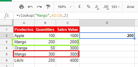
You can use Vlookup to search down the first column in a range with a search key. If the matching value found, the formula would return the value of a specific cell in the same row where the matches found.

Below Vlookup formula returns the result 200. It is the value in the second column of the first occurrence of the Search Key “Mango” in Cell A3.

It repeats the second time in cell A5. But we can’t use Vlookup to find it in the normal way.

But you can do that with a combination of formulas where Google Sheets SMALL function can play a vital role. How?

Here you are going to learn the role of SMALL function in such lookup, not how to use the SMALL function for lookup.

Thought the normal purpose of the SMALL function is to return the Nth Lowest value in a range, we can use it to return Nth Occurrence of a Text or Numeric Value in a range. Then this value you can use in dynamic Vlookup and those steps you can find below. To learn the DYNAMIC VLOOKUP go to our dedicated tutorial HERE.

Use of SMALL Function to Return Nth Occurrence of a Text String  

See the above small data set. Here you can see one item “Mango” repeated twice. With Vlookup, you can use the Search Key as “Mango” and look for the first occurrence of this. That’s in Cell A3. There is no way to look for the second occurrence in Cell A5.

What Google Sheets Small formula can do in this case. It can return the relative position of the second, third or nth occurrence of the repeated item. Here is that trick.

=ArrayFormula(SMALL(IF("Mango"=A2:A6,ROW(A2:A6)-1),2))

We can use the same above small data set. This formula, for example in Cell D6, returns the value 4. which is the relative position of “Mango” in cell A5, which is the second occurrence of that item.

To find the first occurrence, just change the number 2 to 1 in the last part of the above formula. See that modified formula below.

=ArrayFormula(SMALL(IF("Mango"=A2:A6,ROW(A2:A6)-1),1))

This formula returns the answer 2, which is the relative position of the first occurrence of the item “Mango”.

Here is the Break up of the formula used.

Here in the above example, I’ve used two formulas in combination with the SMALL function. They are Google Sheets IF Logical function and ROW function.

Part 1: ROW formula

If you extract the ROW formula part from the above, it will be as follows.

=ArrayFormula(ROW(A2:A6)-1)

Here “A2: A6” is the range. The above formula without “-1” at the end will return the row numbers of the items in the range.

For example 2 for Apple, 3 for Mango and so on. But we need the relative position like Apple 1, Mango 2 likewise.

To do that I’ve applied a “-1” at the end of the formula. You should change this number to “-2” if your range is A3: A7. Hope you understood.

Part 2: IF formula

Now we can use IF function with this ROW formula to return the row number, if the logical expression “Mango” is found, or else to return “False”.

=ArrayFormula(IF("Mango"=A2:A6,ROW(A2:A6)-1))

The result of the above formula will be as below.

Here in this formula result, 2 and 4 are the relative position of “Mango” in the range. Now see the below two formulas which I’ve already mentioned above.

=ArrayFormula(SMALL(IF("Mango"=A2:A6,ROW(A2:A6)-1),1))

This formula returns the number 2, which is the first occurrence of item “Mango”

=ArrayFormula(SMALL(IF("Mango"=A2:A6,ROW(A2:A6)-1),2))

This formula returns the number 4, which is the second occurrence of item “Mango”

You can use this part to create Dynamic Lookup in Google Spreadsheet.