The REPT function has many uses in Google Sheets though the core purpose is to repeat a specified character or string N times.

If you ask me for two real-life examples, two formulas come to mind.

I’ve used it with Vlookup to duplicate rows, and another instance is for creating a Percentage Progress Bar in Google Sheets.

In short, you may find the REPT function helpful when you use it with the functions such as Vlookup, Len, ArrayFormula, Countif, etc.

REPT Function Syntax and Arguments in Google Sheets

Syntax:

REPT(text_to_be_repeated, number_of_repetitions)

Arguments:

text_to_be_repeated – To specify the character or string that you want to repeat.

number_of_repetitions – A positive number specifying the number of times (n) to repeat the text_to_be_repeated.

Google Sheets says it’s limited to 32,000 characters (please refer to the official documentation here).

Both the above arguments can be cell references or hardcoded within the formula.

REPT Function Basic Examples in Google Sheets

First, see some basic examples of the REPT function in Google Sheets.

=rept("-",10)

It repeats the hyphen character ten times.

If you enter the hyphen in cell A1, use the formula below.

=rept(A1,10)

We can use characters directly within the formula or the Char function to convert Unicode numbers and use them.

The character code of the red question mark is 10067. You can use either of the below formulas to get it repeated thrice.

=rept("❓",3)

Or

=rept(char(10067),3)

As a side note, to get several characters, you can use the following ArrayFormula, Sequence, and Char combo in cell A1 in an empty column A.

=ArrayFormula(char(sequence(1000,1,10000)))

In the following example, I have combined two REPT formulas to return black and white stars.

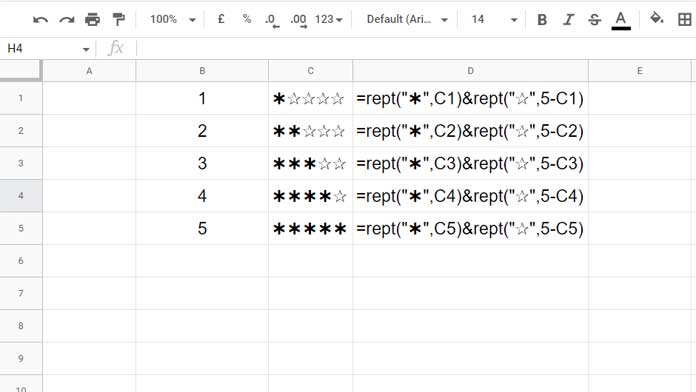
I hope the formulas themselves are self-explanatory.

Practical Use

Other than the two real-life use cases of the REPT function in Google Sheets mentioned at the beginning of this tutorial, here are two more examples.

One example involves Countif and the other with Split and ArrayFormula combination.

Example 1 – Countif in number_of_repetitions

Here I have a list of participants in a painting competition.

You can see their participation status visualized in column G with the help of asterisks.

=rept("*",countif(B3:F3,"Y"))

text_to_be_repeated – *

number_of_repetitions – countif(B3:F3,"Y")

In this example, the Countif counts the occurrences of “Y” in the range B3:F3. It returns 5 for the first row. So the REPT function repeats the “*” 5 times.

I’ve copy-pasted the formula down.

Split and ArrayFormula Combination with REPT

Sometimes we may want to repeat columns N times for printing purposes.

Assume we have generated barcodes for a few items in a column and want it to print N times.

In that case, we can use the REPT function to repeat the column.

The below basic example will give you an idea of using the REPT function in Google Sheets with Split and ArrayFormula combination.

=ArrayFormula(split(rept(A2:A7&";",4),";"))

In the above example, the combination of functions repeats the text and numeric values in column A 4 times.

Formula Explanation:

First, see the REPT formula part.

=ArrayFormula(rept(A2:A7&";",4))

What does it do?

The above formula converts the source data similar to the below image.

Then, we used the Split function to split the text into multiple columns using “;” as the delimiter. That’s all.

I will be back with a few more advanced use of the REPT function in coming tutorials. I hope you have enjoyed this session.