This post is all about the Google Sheets ISERROR function.

There are a few functions in Google Sheets that you can use to find and remove errors: IFERROR, ISERROR, ISERR, IFNA, and ISNA. In this post, we will focus on the ISERROR function, which is specifically used to find errors in Google Sheets.

To remove errors, you may need to use the IF or IFS function with ISERROR. We will discuss this topic in a later part of this tutorial.

Syntax and Arguments

The syntax for the ISERROR function is as follows:

ISERROR(value)

Arguments:

value: The value or expression to be checked for errors. This can be a cell reference, a formula, or a hardcoded value.

The formula returns:

• TRUE if the value is any error, including #DIV/0!, #N/A, #NAME?, #NULL!, #NUM!, #VALUE!, and #REF!.
• FALSE if the value is not an error.

How to Use the ISERROR function in Google Sheets

You can quickly learn how to use the Google Sheets ISERROR function with the help of the following examples.

Basic Formula Examples

Example #1

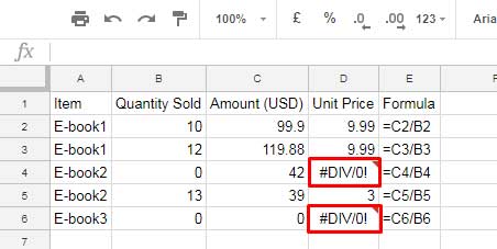
In the following example, two formulas return a #DIV/0! error because the divisor is 0 (zero):

=C4/B4
=C6/B6

Solution:

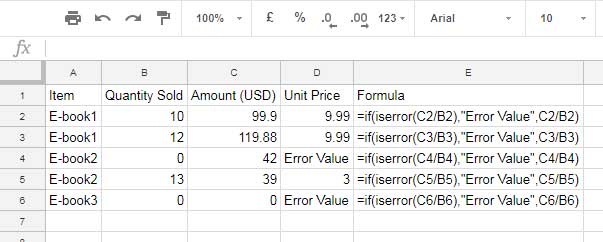
You can use the Google Sheets ISERROR function to return a custom text in the cells that contain errors. For example, the following formula will replace the error value with the text “ERROR VALUE”:

=IF(ISERROR(C2/B2),"ERROR VALUE",C2/B2)

To use this formula, simply insert it into cell D2 and drag it down to cell D6.

Explanation:

The ISERROR function returns TRUE if the value in the expression (formula result) is an error, and FALSE otherwise.

The IF function will return the text “ERROR VALUE” if the ISERROR function returns TRUE, which means that the result of the formula =C2/B2 is an error. Otherwise, the IF function will return =C2/B2.

You can customize the error value returned by the formula by changing the text in the second argument of the IF function. For example, you could change the text to “Divide by zero error” or “Invalid data”.

Update:

We can improve the performance of the IF and ISERROR combination by using the LET function. This avoids the repeated calculation of C2/B2 in the formula.

=LET(calc,C2/B2,IF(ISERROR(calc),"ERROR VALUE",calc))

You can use the LET function in any formula where you need to avoid repeating a calculation.

Example #2: Using ISERROR with VLOOKUP

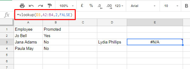
In the following vertical lookup formula, the lookup value (search key) “Lydia Phillips” is not available in the first column of the range A2:A4. For this reason, the VLOOKUP returns a #N/A error:

=VLOOKUP(D3,A2:B4,2,FALSE))

You can use the Google Sheets ISERROR function with VLOOKUP to handle this error as follows:

=ISERROR(VLOOKUP(D3,A2:B4,2,FALSE))

Since the value is an error, ISERROR returns TRUE. You can then use the IF function to return a custom message instead of TRUE, as shown in the following example:

=IF(ISERROR(VLOOKUP(D3,A2:B4,2,FALSE)),"Not found",VLOOKUP(D3,A2:B4,2,FALSE))

Updated With LET:

=LET(calc, VLOOKUP(D3,A2:B4,2,FALSE), IF(ISERROR(calc),"Not found",calc))

Example of Using the ISERROR Function in an Array Formula to Handle Errors

The ISERROR function is a powerful tool for handling errors in Google Sheets. It can be used in conjunction with the ArrayFormula function to apply the ISERROR function to multiple cells at once.

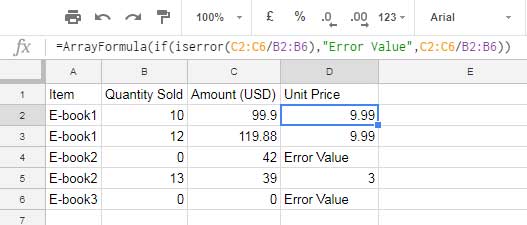
The following formula uses the ISERROR function in an array formula to replace error values in the range C2:C6 with the text “ERROR VALUE”:

=ArrayFormula(IF(ISERROR(C2:C6/B2:B6),"ERROR VALUE",C2:C6/B2:B6))

This formula is equivalent to the following array formula, but it is more efficient because it avoids the repeated calculation of C2:C6/B2:B6:

=ArrayFormula(LET(calc,C2:C6/B2:B6,IF(ISERROR(calc),"ERROR VALUE",calc)))

Difference Between ISERROR and IFERROR in Google Sheets

The ISERROR and IFERROR functions in Google Sheets are both used to handle errors, but they have different purposes.

• ISERROR: The ISERROR function returns TRUE if the value in the specified cell is an error, and FALSE otherwise.
• IFERROR: The IFERROR function returns the value in the specified cell if it is not an error, and a different value if it is an error.

Use ISERROR to:

• Test whether a value is an error.
• Use it with COUNTIF to count the number of error values in a range or in an array formula result.
• Highlight error cells using conditional formatting.
• Optionally mask an error using it with the IF function.

Use IFERROR to:

• Mask an error.
• Return a different value if a formula returns an error.

Example of using ISERROR to count the number of error values returned by an array formula:

=COUNTIF(ArrayFormula(ISERROR(B2:B8/C2:C8)),TRUE)

This COUNTIF formula will return the number of TRUE values returned by the ISERROR formula.